A qubit is not "0 and 1 at the same time"

If you have read anything about quantum computing, you have probably seen the line “a qubit can be 0 and 1 at the same time.” It usually comes right before “so a quantum computer can try every answer at once.”

The first sentence is fuzzy. The second one is wrong. And the fuzziness of the first is what makes the second sound reasonable.

Scott Aaronson has a line at the top of his blog saying that quantum computers won’t solve hard problems by just trying all solutions in parallel.¹ I have been learning quantum computing on my own this year, and the thing that finally made it click was dropping the “both at once” picture entirely and replacing it with a few small pieces of linear algebra. Honestly, the “both at once” version confused me for longer than the math did.

So this post is the explanation I wish I had started with. It is also groundwork. I want to write about Grover’s algorithm next, and Grover makes no sense unless the words “amplitude” and “interference” already mean something to you.

Start with a coin

Here is a fair coin that has been flipped but not looked at. You could describe it as a list of two numbers:

P(heads) = 0.5
P(tails) = 0.5

Those numbers are probabilities. They are between 0 and 1, and they add up to 1. Nobody says the coin is “heads and tails at the same time.” It is one of them, and you just don’t know which. The list describes your knowledge.

Now say you have a process that acts on the coin. “Flip it again” takes any list (p, 1 - p) and turns it into (0.5, 0.5). You can write that as a matrix that multiplies the list. Every classical random process is like this: a matrix with nonnegative entries whose columns sum to 1, acting on a vector of probabilities.

One property matters a lot here. Probabilities can only pile up. If there are two ways to reach “heads,” their probabilities add. They can never subtract. Doing more random stuff to a coin can never make an outcome less likely by having two routes to it cancel out.

Keep that in mind, because it is exactly the property a qubit breaks.

A qubit is a list of amplitudes

A pure qubit state is described by a list of two numbers. We write it like this:

|psi> = a|0> + b|1>

|0> and |1> are just labels for the two basis states, the same way heads and tails are labels. The numbers a and b are called amplitudes. Here is how they differ from probabilities:

1. They can be negative. In general they can be complex numbers.
2. The rule is that their squared magnitudes add up to 1: |a|^2 + |b|^2 = 1.

That second rule says the qubit’s state is a unit vector. IBM’s free course on quantum information describes quantum states exactly this way: column vectors of complex numbers, unit vectors with respect to the Euclidean norm.²

Aaronson’s way of putting it is the one that stuck with me. Classical probability lives in the 1-norm: the entries add up to 1. Quantum mechanics is what you get if you build the same kind of theory on the 2-norm instead, where the squares add up to 1, and then allow minus signs.³ He calls quantum mechanics a generalization of probability theory to allow minus signs. Once you see it that way, a lot of the mystery turns into bookkeeping.

Measurement

So where do probabilities come in? When you measure the qubit in the standard basis, you get 0 with probability |a|^2 and 1 with probability |b|^2. That is the Born rule, from Max Born’s 1926 paper on scattering.⁴ After measuring, the state is just |0> or |1>, whichever you saw. The amplitudes are gone.

This is the step that kills the “try every answer at once” story. Say you have n qubits. Their joint state has 2^n amplitudes, which really is a huge amount of bookkeeping. But when you measure, you get one n-bit string out. That’s it. You don’t get to read the amplitudes. You get a single sample.

There is a theorem that makes this precise. Holevo’s bound from 1973 says that n qubits can’t carry more than n classical bits of information you can actually retrieve.⁵ All those 2^n numbers are real in the sense that they affect what happens. They are just not something you can read out.

So if “both at once” meant “the computer gets to see both answers,” it would be false. The only thing a quantum algorithm can do is arrange for the amplitude of the right answer to be large when you finally measure. That brings us to interference.

Interference is the whole trick

Because amplitudes can be negative, two paths to the same outcome can cancel. That is interference, and it is the reason quantum computing is different from “a coin flip with extra steps.”

The cleanest place to see it is the Hadamard gate, written H. As a matrix:

H = 1/sqrt(2) * [[1,  1],
                 [1, -1]]

It acts on the basis states like this:

H|0> = (|0> + |1>) / sqrt(2)    = |+>
H|1> = (|0> - |1>) / sqrt(2)    = |->

These two output states have names, |+> and |->. Now look at what happens if you measure either one. Both give 0 with probability 1/2 and 1 with probability 1/2, because (1/sqrt(2))^2 = (-1/sqrt(2))^2 = 1/2. Measured in the standard basis, they give the same probabilities.

But they are not the same state. The IBM course makes this point directly: measured right away, |+> and |-> look identical, but apply H again first and you can tell them apart perfectly.²

The worked example

Start with |0>. Apply H once:

|0>  --H-->  (1/sqrt(2))|0> + (1/sqrt(2))|1>

If this were a coin, you would now have a fair 50/50 coin. Flip a fair coin again and it stays 50/50. So let’s apply H again and see if the qubit agrees.

Apply H to each piece separately (it is linear, so that’s allowed):

(1/sqrt(2)) * H|0> = (1/sqrt(2)) * (1/sqrt(2)) * (|0> + |1>) = 1/2 |0> + 1/2 |1>
(1/sqrt(2)) * H|1> = (1/sqrt(2)) * (1/sqrt(2)) * (|0> - |1>) = 1/2 |0> - 1/2 |1>

Now add them up:

|0>:  1/2 + 1/2 = 1
|1>:  1/2 - 1/2 = 0

You are back at |0>, with certainty. The two paths that lead to |0> have the same sign and add up. The two paths that lead to |1> have opposite signs and cancel.

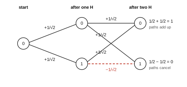
This is the picture I want you to keep. The randomizing coin process above cannot do this. Its paths carry nonnegative probabilities, so they cannot cancel in the way these amplitudes do. A qubit can, because of one minus sign.

Notice what this says about the “both at once” story. After the first H, the qubit is in an equal superposition. If superposition meant “it is secretly 0 or secretly 1, we just don’t know,” the second H would leave it at 50/50, like the coin. It doesn’t. If superposition meant “it is fully 0 and fully 1 and the computer gets both,” that also doesn’t explain why the result is exactly |0>. What explains it is that the state is a vector with signed entries, and gates combine those entries the way matrices do.

You can check this in a few lines of Qiskit:

from qiskit import QuantumCircuit
from qiskit.quantum_info import Statevector

qc = QuantumCircuit(1)
qc.h(0)
print(Statevector(qc).probabilities())  # [0.5 0.5]

qc.h(0)
print(Statevector(qc).probabilities())  # [1. 0.]

# Start from |1> instead: the minus sign moves to the other side
qc2 = QuantumCircuit(1)
qc2.x(0)
qc2.h(0)
print(Statevector(qc2))                 # [ 0.707, -0.707]
qc2.h(0)
print(Statevector(qc2).probabilities()) # [0. 1.]

I ran this on a simulator and got those outputs (up to floating point rounding). The Statevector class lets you peek at the amplitudes, which you can only do because it is a simulation. On real hardware you’d only see measurement counts.

The Bloch sphere

There is a nice way to picture all possible states of one qubit. Since |a|^2 + |b|^2 = 1, and an overall phase on the whole state doesn’t change anything you can measure, you can always write a single-qubit state as:

|psi> = cos(theta/2)|0> + e^(i*phi) sin(theta/2)|1>

Two angles, theta and phi. Two angles pick out a point on a sphere. That sphere is the Bloch sphere, named after Felix Bloch, who used this kind of geometry for spinning nuclei in a magnetic field in 1946.⁶ Nielsen and Chuang use it as their main picture for single qubits.⁷

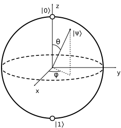
Some things that are hard to say in words become obvious on the sphere:

• |0> is the north pole and |1> is the south pole.
• |+> and |-> sit on the equator, on opposite sides. That is the geometric version of “same measurement statistics, different states.” Measuring in the standard basis only asks how far north or south you are. Both are exactly halfway.
• Every point on the equator gives a 50/50 measurement. There are infinitely many different “equal superpositions,” and they differ in phi. “Both at once” can’t tell any of them apart, but gates can.
• Single-qubit gates are rotations of the sphere. The Hadamard is a 180 degree rotation about the axis halfway between X and Z, which swaps the north pole with |+> and the south pole with |->. Do it twice and you’re back where you started, which is the worked example above in picture form.

One thing that trips a lot of people up: states that are orthogonal as vectors (at 90 degrees to each other), like |0> and |1>, end up on opposite poles of the sphere, 180 degrees apart. That is what the half angle theta/2 in the formula is doing. For pure states, the angle on the sphere is twice the angle defined by the magnitude of their inner product.

The Bloch sphere also has a limit. It only works for one qubit. Two qubits have four amplitudes, and entangled states don’t have a nice “point on a sphere per qubit” picture. So it is a great tool for building intuition about amplitudes and phase, and a bad tool for intuition about what makes multi-qubit algorithms powerful.

Why “both at once” misleads

I want to be fair to the phrase. Superposition does mean the state has nonzero amplitude on both |0> and |1>. If someone says “both at once” as shorthand for that, fine.

The problem is what people do with it next. Here are the three places I think it goes wrong.

It hides the signs. “Both at once” sounds like the same description for |+> and |->, and for every point on the equator. But those states behave completely differently under the next gate. The information that matters most, the relative sign or phase, is exactly the part the phrase throws away.

It suggests you get all the answers. If a register is “every number at once,” it sounds like a function evaluated on it gives you every output at once. You do get a state with all those outputs encoded in amplitudes. Then you measure and get one random output, which is no better than picking one input at random and computing classically. The real work is designing the algorithm so that wrong answers interfere destructively before you measure. That is hard, and for most problems nobody knows how to do it.

It makes quantum speedups sound unlimited. If you really got to try everything in parallel, any search over N options would take one step. It doesn’t. Grover’s algorithm searches N items in about sqrt(N) steps,⁸ and a 1997 result showed no quantum algorithm can do unstructured search with fewer queries than that, up to a constant.⁹ A square-root speedup is great. It is also very different from “instant.” Aaronson’s blog tagline exists because this misunderstanding keeps showing up.¹

Aaronson and Zach Weinersmith made an SMBC comic about this in 2016 called “The Talk,” framed as a parent sitting a kid down to explain how quantum computing really works.¹⁰ It is the funniest version of this argument I know, and it makes the same point: the power comes from amplitudes interfering, and you have to choreograph that interference so the right answer survives.

What to keep

What I find strange and exciting is that the amplitudes can change what happens when we bring paths back together. A measurement only gives us an outcome, but the steps before it let us arrange which outcomes become more or less likely.

That makes the next question much more concrete for me: how can we arrange those steps to solve a problem? Grover’s algorithm is a good place to explore that. It turns interference into something we can calculate and watch, while also showing why having many possible outcomes doesn’t mean we get to read them all.

If you want to go further

Here is what I’d read, in this order:

1. IBM’s free “Basics of Quantum Information” course.² It starts with classical probability vectors and builds quantum states on top of them, which is the framing in this post. It is careful and doesn’t skip steps.
2. Aaronson’s Lecture 9 from Quantum Computing Since Democritus.³ It is short, funny, and the 1-norm versus 2-norm argument is in there.
3. Nielsen and Chuang, chapters 1 and 2, once you’re comfortable with matrices.⁷ It is the standard textbook for a reason.

And honestly, just run the Qiskit snippet above. Change the starting state, add a third H, put a z gate between the two Hadamards and see what happens. (Spoiler: the z flips the sign on |1>, so the cancellation moves and you end up at |1>.)

Sources