Attention Is All You Need, read in 2026

“Attention Is All You Need” is one of the most cited machine learning papers ever, but my familiarity with it was mostly secondhand. I knew the diagram. I knew “queries, keys, values.” I did not know what the paper actually argued, what problem it thought it was solving, or which parts of it are still sitting inside the models we use every day.

So I sat down and read the whole thing, the arXiv version, with one question in my head: if you read this in 2026, knowing everything that came after, what holds up?

The short answer is that the core idea held up almost perfectly, a lot of the specific choices got swapped out, and the paper did not explore the scale its architecture would later reach.

What the paper actually says

The first surprise is how narrow the paper is. It is a machine translation paper. The abstract says the Transformer is “based solely on attention mechanisms,” and then spends most of its energy on English-to-German and English-to-French translation scores.¹

The setup in 2017 was this. The best translation systems were encoder-decoder models built on recurrent networks (RNNs) or convolutions, with attention bolted on so the decoder could look back at the source sentence. Attention itself was not new. Bahdanau, Cho and Bengio had introduced it for translation in 2014, as a way to stop squeezing a whole sentence into one fixed-size vector.² The Transformer’s move was to delete the recurrence entirely and keep only the attention.

The reason they gave was mostly about speed. An RNN processes a sentence one word at a time, because each step needs the previous step’s hidden state. That is a sequential bottleneck you cannot throw more GPUs at. Self-attention connects every position to every other position in a constant number of sequential steps, so the whole sentence can be processed in parallel.¹

The paper’s own comparison table makes this concrete. Per layer, self-attention costs O(n² · d) and a recurrent layer costs O(n · d²), where n is sequence length and d is the size of each token’s vector. The authors point out that self-attention is cheaper when n is smaller than d, “which is most often the case” for sentence-level translation.¹ Hold onto that line. It comes back later.

The numbers they reported:

• 28.4 BLEU on WMT 2014 English-to-German, more than 2 BLEU above the previous best, including ensembles.
• 41.8 BLEU on WMT 2014 English-to-French for a single model.
• The big model trained for 3.5 days on one machine with 8 NVIDIA P100 GPUs. The base model trained for 12 hours.¹

The base model had 6 layers in the encoder, 6 in the decoder, a model width of 512, 8 attention heads, and about 65 million parameters. The big one had about 213 million.¹

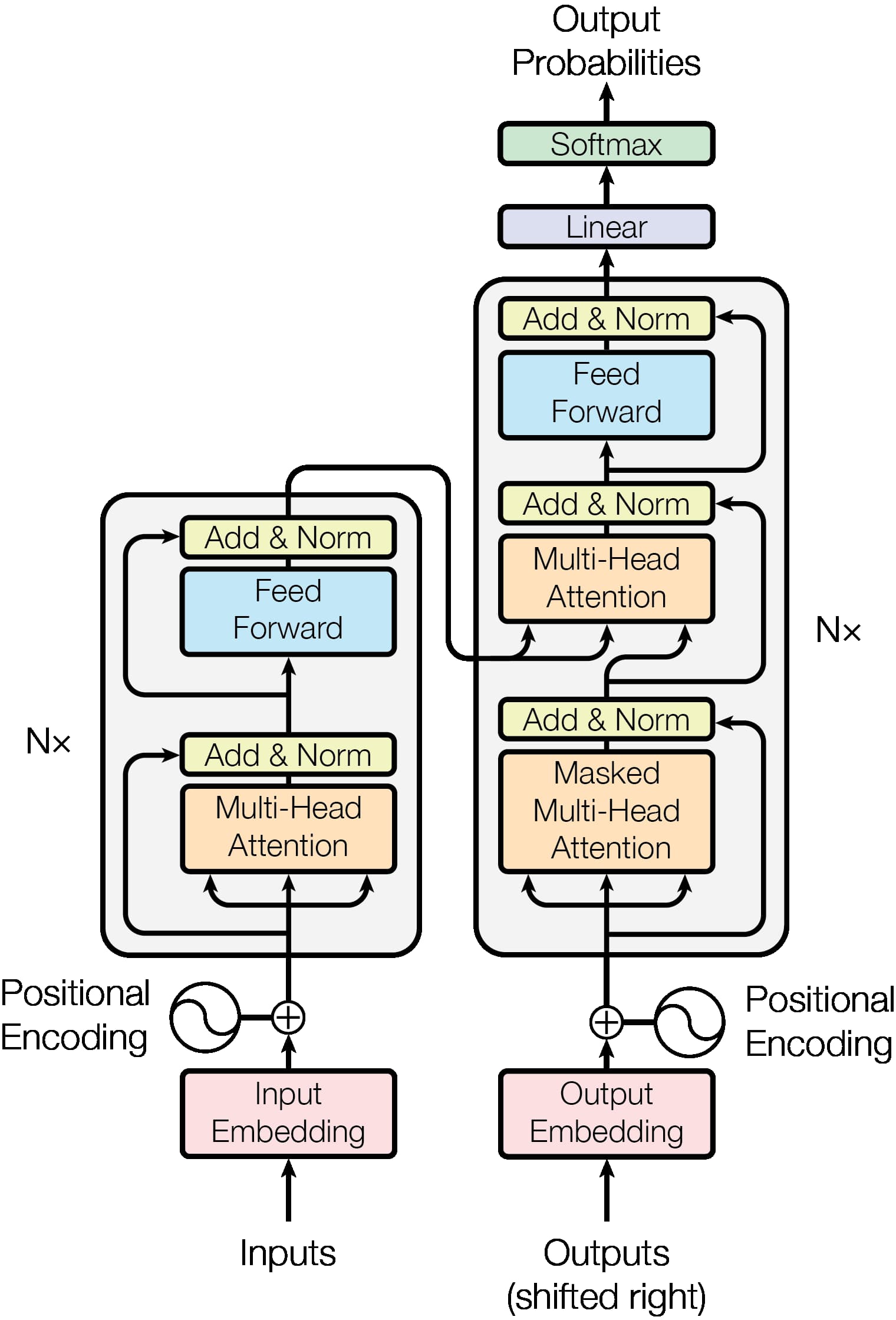
If you look at that diagram with 2026 eyes, a few things jump out. There are two stacks. There is a little sine wave next to the inputs. And “Add & Norm” sits on top of every block. Each of those three details has a different story.

What survived

Attention itself

Scaled dot-product attention is the same today as it was in the paper:

Attention(Q, K, V) = softmax(Q Kᵀ / sqrt(d_k)) V

Every token makes a query, every token makes a key and a value, each query scores every key, the scores go through a softmax, and the output is a weighted average of the values. The sqrt(d_k) is there because dot products of big vectors get big, and a softmax over big numbers turns into a hard one-hot pick with tiny gradients. That fix is still standard.

Multi-head attention also survived. Instead of one attention with width 512, you run 8 smaller ones of width 64 in parallel and concatenate them. The ablation table in the paper is honest about how much this matters: a single head was 0.9 BLEU worse than the best setting, and too many heads also hurt.¹ So it helps, but it is not magic, which is a pretty fair summary of most architecture choices.

One detail I liked: when they shrank the key dimension, quality dropped, and they wrote that “a more sophisticated compatibility function than dot product may be beneficial.”¹ Nine years later, the dot product is still the compatibility function. The hunch did not pan out, or at least nobody found the better function that also runs fast on a GPU.

The part of attention that did change is the bookkeeping around keys and values. When you generate text one token at a time, you cache every past key and value, and that cache gets huge. Tricks like grouped-query attention, where several query heads share one set of keys and values, exist mostly to shrink that cache.³ That is an inference-cost problem the 2017 paper never had to think about, because translating one sentence at a time does not stress memory the way a long chat does.

Residual connections

Every sublayer in the Transformer is wrapped in a residual connection: the output is x + Sublayer(x), so the sublayer only has to learn a change to its input, not a whole new representation. The paper took this directly from ResNet, which introduced residual learning for very deep image networks in 2015.⁴¹

This is the part of the architecture I think about most. Because every layer adds into the same running vector, you can think of a Transformer as a stream of information that each layer reads from and writes to. That “residual stream” view is basically the foundation of a lot of interpretability work now. The 2017 paper does not frame it that way at all. It just says residuals help train deep networks. But the choice to make everything additive is a big reason the inside of these models is even somewhat readable.

Normalization (sort of)

Layer normalization, from Ba, Kiros and Hinton in 2016, is in the original paper and is still in every model.⁵ What changed is where it goes and which version is used. That gets its own section below.

The decoder’s causal mask

In the decoder, each position is only allowed to attend to positions at or before itself. The paper implements this by setting the forbidden attention scores to negative infinity before the softmax, so the model cannot peek at the word it is supposed to predict.¹ This tiny trick is a core piece of how every chatbot generates text left to right. It survived completely unchanged.

What got replaced

Sinusoidal positions became RoPE

Attention by itself has no idea about order. “Dog bites man” and “man bites dog” are the same set of tokens. So the paper adds a positional encoding to each input embedding: a fixed pattern of sines and cosines at different frequencies, so each position gets a unique fingerprint.

What surprised me is that the paper itself says this choice barely mattered. They tried learned position embeddings too and “found that the two versions produced nearly identical results.” They picked sinusoids because they “may allow the model to extrapolate to sequence lengths longer than the ones encountered during training.”¹

That hope did not really hold. When Press, Smith and Lewis studied length extrapolation in 2021, they found that the position methods in use at the time did not allow efficient extrapolation to longer inputs, which is why they proposed a different scheme called ALiBi.⁶

A widely adopted alternative is rotary position embedding, or RoPE, from Su et al. in 2021. Instead of adding a position vector to the token, RoPE rotates the query and key vectors by an angle that depends on position. When you take the dot product of a rotated query and a rotated key, the result depends on how far apart they are, so relative position falls out of the math for free.⁷ When Meta released LLaMA in 2023, they listed “Rotary Embeddings” as one of three changes from the original Transformer, removing absolute position embeddings entirely.⁸ A lot of open models since then have followed that lead.

I find this one funny. The paper’s stated reason for its choice was the one property that turned out not to work, and the thing that replaced it is still built on sines and cosines. Rotation by an angle is just sines and cosines wearing a different hat.

Post-norm became pre-norm

Here is the exact line from the paper: the output of each sublayer is LayerNorm(x + Sublayer(x)).¹ The normalization happens after the residual add. That is called post-norm.

Many large language models use the other order: x + Sublayer(Norm(x)). Normalize the input to the sublayer, and leave the residual path untouched. That is pre-norm.

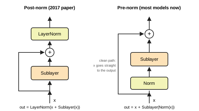
The reason is training stability. Xiong et al. showed in 2020 that with post-norm, the gradients near the output layer are large at initialization, so you need a careful learning-rate warm-up to avoid blowing up. With pre-norm, gradients are well behaved at the start, and they could train without the warm-up at all.⁹

This connects to something in the original paper that I skimmed past the first time. The learning rate schedule increases linearly for the first 4,000 steps, then decays.¹ That warm-up was not decoration. With post-norm, it was holding the whole thing together.

Pre-norm also fits the residual stream picture better. In the right half of that diagram, the original input flows straight to the output, and each layer just adds something. In post-norm, every layer rescales the whole stream.

The norm itself also changed. LLaMA uses RMSNorm, from Zhang and Sennrich in 2019, which skips subtracting the mean and only divides by the root-mean-square.¹⁰⁸ It is cheaper and seems to work just as well.

The feed-forward block got a gate

The original feed-forward layer is two matrix multiplies with a ReLU in between: max(0, xW1 + b1)W2 + b2, with an inner width of 2048.¹ Shazeer showed in 2020 that gated variants, where one linear projection multiplies another after an activation, gave better results in his experiments, and one of them, SwiGLU, is now standard.¹¹ LLaMA lists it right next to pre-norm and RoPE.⁸ This is the least famous change and maybe the most boring, which is kind of the point. Changes like this account for some of what separates later models from the original design.

Encoder-decoder became decoder-only

The diagram has two towers. Most models people talk about in 2026 have one.

The original design made sense for translation. You have a source sentence, an encoder reads all of it in both directions, and a decoder writes the target sentence while attending back to the encoder. Two different jobs, two stacks.

Within about a year, people started pulling the towers apart. OpenAI’s first GPT, in 2018, was a 12-layer decoder-only Transformer, trained to predict the next token on a big pile of books and then fine-tuned for other tasks.¹² BERT went the other way and kept only the encoder, trained to fill in masked words.¹³ Encoder-only models are still everywhere for search and classification. But for generation, the decoder-only design won, and it won because of how simple it is. Everything is a sequence. The prompt and the answer are the same stream of tokens. There is no separate source and target, so there is nothing to design around.

In my view, this is the change that matters most for how we think about these models now. Once the source and the target are one sequence, “translation” becomes a special case of “continue this text,” and so does almost everything else.

The benchmarks

The paper’s headline numbers are WMT 2014 BLEU scores. BLEU measures word overlap between a model’s translation and a reference translation.

I cannot remember the last time I saw a big model release lead with a WMT BLEU score. The things people measure now, like reasoning, coding, and following instructions, are things the 2017 setup was not even trying to do. I do not think that makes the old numbers worthless. They did their job: they convinced people the architecture was worth trying. But reading the results section in 2026 feels a bit like reading the lap times of a car that later got turned into an airplane.

What it under-sold: scale

This is the part I think matters most.

The paper frames parallelism as a way to train faster and cheaper. The big model trained for 3.5 days on 8 GPUs, at “a small fraction of the training costs” of the competition.¹ That is the selling point. Same quality or better, less compute.

Six years later, the LLaMA paper reported training its 65-billion-parameter model on 2,048 A100 GPUs for about 21 days, over roughly 1.4 trillion tokens.⁸ That model is about 300 times bigger than the 2017 big model, and it is not even close to the largest model trained since.

What happened in between is that people realized the parallelism did more than make things cheaper. It made it possible to keep going. Kaplan et al. at OpenAI showed in 2020 that language model loss falls as a smooth power law in model size, dataset size, and compute, with some trends spanning more than seven orders of magnitude.¹⁴ Hoffmann et al. at DeepMind followed up in 2022 with the Chinchilla paper, arguing that most large models were undertrained and that model size and training tokens should be scaled up together.¹⁵

The Transformer is the architecture that made those curves easy to ride. An RNN has to process tokens one after another, so you hit a wall on how much data you can push through per second. A Transformer does the whole sequence at once during training, which maps really well onto GPUs that are basically giant parallel matrix multipliers.

To be fair to the authors, the conclusion is not narrow at all. They wrote that they planned to extend the Transformer to “input and output modalities other than text” and to handle “images, audio and video.”¹ That happened. Transformers now show up in vision, speech, and video models too. So they saw the breadth.

What I do not see anywhere in the text is the idea that you would make the thing a thousand times bigger and get qualitatively new behavior out of it. The paper is a very good engineering paper about translation. As far as I can tell from reading it, nobody was claiming in 2017 that it had accidentally described the engine for everything after.

The line that aged worst

Remember the complexity argument? Self-attention costs O(n² · d) per layer, and the authors said that is fine because n is usually smaller than d for sentences.¹

For a translation sentence of maybe 30 tokens and a model width of 512, that is true. For a model reading a whole codebase, or a long legal document, n is in the tens or hundreds of thousands and d is a few thousand. The quadratic term that did not matter in 2017 is now one of the main things people engineer around.

I ran into a small version of this with DebateSim, where the platform has to handle bills that run past 40,000 characters. The paper itself suggested restricting attention to a local neighborhood of size r for very long sequences.¹ We dealt with it at the application level by pulling out the sections that matter, which is a much cruder cousin of the same idea. Variants of restricted attention are among the ways people handle long context now.

Reading it as a 2026 reader

Reading this now, I keep coming back to how much grew out of a fairly specific design choice. The paper was trying to make sequence modeling work better without recurrence. It wasn’t a complete plan for everything people would later ask language models to do.

That makes me curious about the choices we treat as obvious today. Some parts of this architecture have lasted, while others have changed as models and training runs grew. Which current defaults will look just as temporary in a few years? I don’t know, but reading the original paper makes it easier to imagine that the next useful change could begin with a similarly concrete problem.

Sources