Grover's algorithm, explained with a phone book

This is how Grover’s algorithm finally made sense to me, written the way I wish someone had explained it. I used to hear “quantum computers search a database in square root time” and assume the quantum computer was checking every entry at once. It isn’t. What it actually does is weirder and, honestly, a lot more fun once it clicks.

So let’s start with a phone book.

The backwards phone book problem

A phone book is sorted by name. If I give you a name, you can find the number fast. Open to the middle, see if you are too far or not far enough, cut the book in half, repeat. For a million entries that takes about 20 looks.

Now flip it. I give you a phone number and ask whose it is. The sorting is useless now. The number could be on any page. Without another index or useful structure, you have to check entries until you find it.

If there are N entries and exactly one matches, on average you read about half of them before you find it. Grover’s original paper puts it this way: any classical algorithm needs to look at about N/2 entries to have even a 50% chance of finding the target.¹ For a million entries that is roughly 500,000 looks.

This is called unstructured search. You have a yes/no checker (is this the right number?) and nothing else. No ordering, no hints, no partial credit.

Grover showed that a quantum computer can solve this with about sqrt(N) uses of the checker.¹ For a million entries, about 785 instead of 500,000. The factor that gives 785 will come from the geometry below.

The setup, in plain terms

With n qubits you can represent N = 2^n entries. Each entry gets a label, like 00, 01, 10, 11 for 4 entries. The quantum state is a list of N numbers called amplitudes, one per entry. When you measure, you get entry x with probability equal to its amplitude squared.

The game is simple to state. Start with every amplitude equal, so every entry is equally likely. Then somehow pump the target’s amplitude up and everyone else’s down, so that when you measure, you almost certainly get the target.

The checker becomes a quantum oracle. You feed it a superposition of entries and it flips the sign of the target’s amplitude, leaving everything else alone. That’s all it does. It doesn’t tell you which one it flipped. A sign flip by itself doesn’t change any probability, because (-a)^2 = a^2. If you measured right after the oracle, you’d learn nothing.

The trick is the second step.

Reflect about the mean

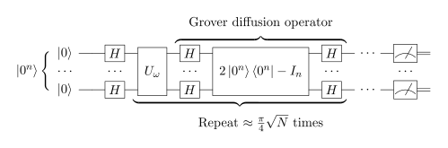
The second step is called the diffusion operator, and the cleanest way I know to describe it is: take every amplitude and reflect it about the average.

new_amplitude = 2 * mean - old_amplitude

If an amplitude was a little above the mean, it ends up a little below. If it was far below the mean, it ends up far above.

Now put the two steps together. Every entry starts at the same small positive amplitude. The oracle flips the target to negative. That drags the mean down a tiny bit, but the target is now way below the mean. Reflecting about the mean throws the target way above it, while everyone else drops slightly.

One round of “flip, then reflect” is one Grover iteration. Each iteration moves a bit of amplitude out of the wrong answers and into the right one.

A tiny worked example: 4 entries

Here’s the example that made it click for me, because the numbers come out perfectly.

Four entries, two qubits. The target is 11.

Start. Equal superposition. Each amplitude is 1/2, so each probability is 1/4.

entry:      00     01     10     11
amplitude:  0.5    0.5    0.5    0.5

Oracle. Flip the sign of 11.

entry:      00     01     10     11
amplitude:  0.5    0.5    0.5   -0.5

Mean. (0.5 + 0.5 + 0.5 - 0.5) / 4 = 0.25.

Reflect about the mean. Apply 2 * 0.25 - a to each.

entry:      00     01     10     11
amplitude:  0.0    0.0    0.0    1.0

The three wrong answers go to exactly zero. The target goes to exactly 1. Probability of measuring 11 is 1.0, after a single call to the oracle.

Classically, with 4 entries, you’d need up to 3 looks to be sure (if the first three are wrong, the fourth must be it). The quantum version does it in one. That’s a tiny gap, but it’s the same mechanism that gives 785 versus 500,000 at scale.

The first time I worked this out by hand, I honestly didn’t believe it and re-did the arithmetic. It’s a strangely clean result.

The geometric picture

The amplitude arithmetic works, but it doesn’t tell you why the number of iterations is sqrt(N). For that you need the picture, which is in Nielsen and Chuang and is the version I find most convincing.²

Here’s the key observation. At every point in the algorithm, all the wrong entries have the same amplitude as each other. So you really only need to track two numbers: the target’s amplitude, and the “everyone else” amplitude. That means the state lives in a flat 2D plane, spanned by two directions:

• |w>, the target entry
• |s'>, the even mix of all the wrong entries

The starting state |s> (the even superposition over everything) is almost entirely along |s'>, tilted just slightly toward |w>. Call that small tilt angle theta/2. Since the target’s starting amplitude is 1/sqrt(N):

sin(theta / 2) = 1 / sqrt(N)

Now both steps are reflections in this plane:

• The oracle flips the sign of the |w> component. That’s a reflection across the |s'> axis.
• The diffusion operator is a reflection across the starting state |s>.

Two reflections in a row make a rotation, and the angle of that rotation is twice the angle between the two mirrors. The mirrors are theta/2 apart, so every Grover iteration rotates the state by theta toward the target. Same angle every time.

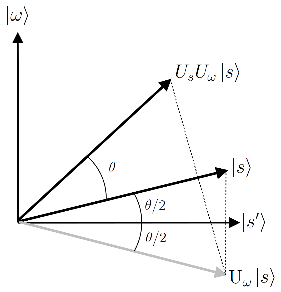
After k iterations the angle from |s'> is (2k + 1) * theta / 2, and the probability of measuring the target is:

P(target after k iterations) = sin^2((2k + 1) * theta / 2)

You want that angle to hit 90 degrees, where the state points straight at |w>. For big N, theta/2 is about 1/sqrt(N), so you need roughly (pi/2) / (2/sqrt(N)) steps:

k ≈ (pi / 4) * sqrt(N)

That’s where the famous (pi/4)sqrt(N) comes from, and why it’s a square root. The rotation per step is proportional to 1/sqrt(N), and you need to cover a fixed 90 degrees.

Check it against the 4-entry example. sin(theta/2) = 1/2, so theta/2 = 30 degrees and each step rotates by 60. One step takes you from 30 to 90 degrees. Exactly on target, which is why the probability came out as exactly 1.

For the million-entry phone book, theta/2 = arcsin(1/1000), which is about 0.001 radians. Plug in and the best number of iterations is 785, with success probability essentially 1.

Over-rotating makes it worse

This is the part that surprises people the most. Grover’s algorithm doesn’t converge. It rotates. If you keep going past 90 degrees, you rotate right past the target and the probability goes back down.

With 4 entries: one iteration gives probability 1. Two iterations put you at 150 degrees, and the probability drops to 0.25, the same as random guessing. For the million-entry book, 785 iterations gives about 1.0, 1,000 iterations gives about 0.83, and 1,570 iterations brings you almost all the way back to 0.

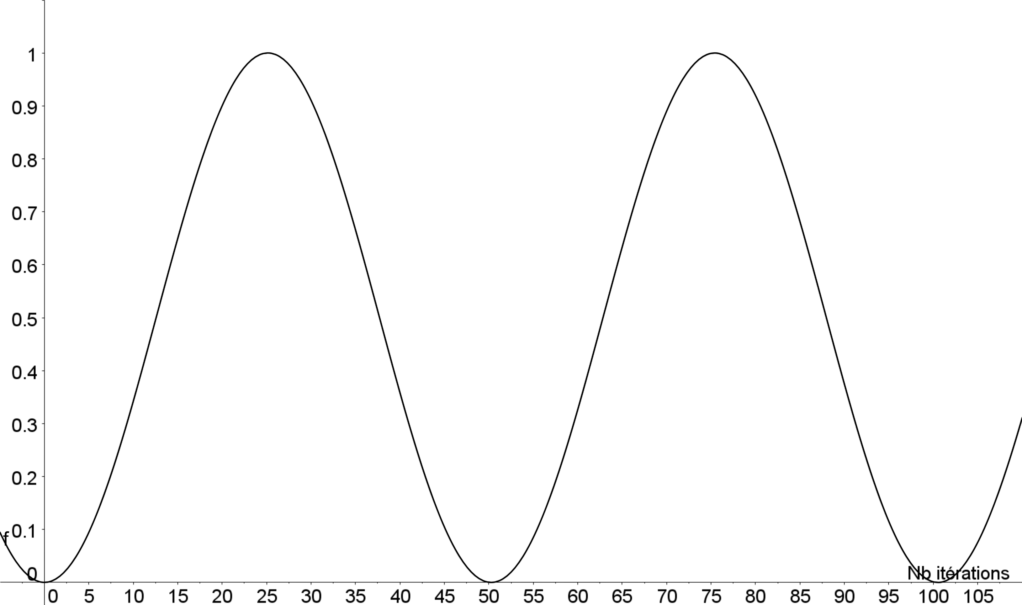
So you need to know (or estimate) how many targets there are, because that sets the rotation angle and therefore when to stop. With M marked entries, sin(theta/2) = sqrt(M/N), and IBM’s Qiskit tutorial computes the stopping point exactly that way: floor(pi / (4 * arcsin(sqrt(M/N)))).³ There are variants that handle an unknown M, but I’m not going to go into them here.

The 2-qubit version in Qiskit

Here’s the 4-entry search as a Qiskit circuit. I checked the API names against the current Qiskit docs and ran it on Qiskit 2.4.⁴⁵

from qiskit import QuantumCircuit
from qiskit.quantum_info import Statevector
from qiskit.primitives import StatevectorSampler

qc = QuantumCircuit(2)
qc.h([0, 1])      # equal superposition over 00, 01, 10, 11

qc.cz(0, 1)       # oracle: flip the sign of |11>

qc.h([0, 1])      # diffusion: reflect about the mean
qc.x([0, 1])
qc.cz(0, 1)
qc.x([0, 1])
qc.h([0, 1])

print(Statevector(qc).probabilities_dict())   # '11' -> ~1.0

qc.measure_all()
result = StatevectorSampler().run([qc], shots=1000).result()
print(result[0].data.meas.get_counts())       # {'11': 1000}

A few notes if you run this yourself:

• The oracle for 11 is just a controlled-Z. CZ multiplies |11> by -1 and leaves the other three alone, which is exactly “flip the sign of the target.”
• The diffusion block is H, X, CZ, X, H. The Xs move the sign flip onto |00>, and the Hs turn “reflect about |00>” into “reflect about the even superposition.” Technically this version is the reflection times -1, a global phase, which doesn’t change any measurement.
• measure_all() names the classical register meas, which is why the counts live at result[0].data.meas.
• For bigger searches, Qiskit has a grover_operator() function in the circuit library that builds the iteration from your oracle, and the IBM tutorial uses it.³ For 2 qubits I’d rather write the gates by hand so you can see every piece.

When I ran it, every one of the 1,000 shots came back 11. That’s the worked example, on a (simulated) quantum computer.

The honest limits

This is where I try to slow down, because Grover is easy to oversell.

It’s quadratic, not exponential

Going from N to sqrt(N) is a big deal for large N. But it’s a different kind of win from what Shor’s algorithm does to factoring, where the quantum speedup is believed to be exponential. If a classical brute force takes 2^128 steps, Grover takes about 2^64. That’s a huge reduction, and still an absurd number.

You can’t do better

This is the part I find beautiful. In 1997, Bennett, Bernstein, Brassard, and Vazirani proved that relative to a random oracle, a quantum computer can’t solve this kind of search in fewer than about 2^(n/2) steps, and that Grover already hits that bound.⁶ Zalka later tightened it and showed Grover’s algorithm is exactly optimal, with about (pi/4)sqrt(N) queries needed for near-certain success.⁷ Grover himself noted in the original paper that his algorithm was within a small constant factor of the best possible.¹

So “quantum computers will make unstructured search exponentially faster” isn’t just unproven. For black-box search, it’s false. The square root is the ceiling.

You need a quantum oracle

The phone book framing hides a real problem. The oracle has to be a quantum circuit that recognizes the target. If your “database” is a big classical list sitting on a hard drive, somebody has to load all N entries into the quantum computer to build that oracle, and that alone costs on the order of N work. At that point you could have just scanned the list. My view is that Grover makes the most sense when the checker is a computation you can write as a circuit (like “does this key decrypt this ciphertext?”) and not a lookup into stored data.

It needs fault-tolerant hardware

Grover’s speedup only shows up when sqrt(N) iterations run one after another, coherently. Zalka showed you can’t parallelize quantum search better than splitting the search space across separate machines.⁷ Splitting a search across P machines means each one searches N/P entries in about sqrt(N/P) steps, so total work grows. For any size that matters, that means millions or billions of sequential gate layers with errors corrected the whole way. That’s a fault-tolerant quantum computer, which nobody has built at that scale yet.

What this means for AES

The most common place Grover shows up in real conversations is symmetric cryptography, so here’s what I’ve learned.

The textbook argument goes like this. Brute-forcing an AES-128 key classically means trying up to 2^128 keys. Grover turns that into about 2^64 iterations, so AES-128 is “effectively 64-bit” against a quantum attacker. AES-256 drops to “effectively 128-bit,” which is still far out of reach. Hence “just use AES-256.” Researchers have worked out what the AES oracle would actually cost as a fault-tolerant circuit, with exact qubit and gate counts for all three key sizes.⁸

The NSA’s CNSA 2.0 suite does specify AES with 256-bit keys, which is NSA policy rather than a statement about Grover.⁹ If you want the most conservative choice, AES-256 is the easy one to defend, and the cost of switching is usually small.

But I want to be honest that NIST’s own position is more relaxed than the “effectively 64-bit” line suggests. NIST’s post-quantum FAQ points out that all of Grover’s steps have to run in series to get the full speedup, and says it expects Grover to give “little or no advantage in attacking AES.”¹⁰ It says AES-128 will stay secure for decades and that applications can keep using 128, 192, or 256-bit keys.¹⁰ NIST’s draft transition plan (IR 8547) is about retiring quantum-vulnerable public-key algorithms like RSA and elliptic curves, not AES.¹¹ Filippo Valsorda wrote a good breakdown of why the parallelization problem makes a Grover attack on AES-128 wildly impractical, using published oracle cost estimates.¹²

My take: the “AES-128 becomes 64-bit” framing is a good way to understand the math, and AES-256 is a reasonable default for anything new that has to last a long time. But the urgent post-quantum work is on public-key crypto, where Shor’s algorithm is the real threat. Grover is a much smaller problem for symmetric keys.

What I’d build next

I’d start with eight entries and plot the chance of getting the marked answer after each iteration. Watching that probability rise and then fall would make the stopping rule much easier to believe than memorizing a square-root formula.

What I find so cool is that the extra iterations can undo the progress. The algorithm only helps when the rotations line up in the right way. That makes me curious about how a useful search problem gets turned into an oracle in the first place, because that construction is part of the work too. The speedup is more interesting once we can see both what creates it and what it costs.

Sources