How a word gets meaning inside a model

A language model never sees the word “bank.” It sees a number, something like 4,173, and that number has no more to do with rivers or money than your locker number has to do with you. Somewhere between that integer and the model’s output, “bank” picks up enough meaning that the model can tell a riverbank from a savings account.

This post is about how that happens. The order I go in (token, then embedding, then the stream of vectors that flows through the layers) is borrowed from 3Blue1Brown’s chapter on transformers,¹ which is worth watching alongside this. I want to go a bit further in two places: the famous king - man + woman = queen trick, which is more fragile than it looks, and the question of what any single number in these vectors actually means. The short answer to that one is “usually nothing on its own,” and the longer answer is one of the more interesting things going on in interpretability right now.

Step one: a word becomes an ID

Before anything else, the text gets chopped into tokens. A token is often a whole common word, sometimes a piece of a word, sometimes a space plus a word. Each token in the vocabulary has an integer ID. GPT-2, for example, has a vocabulary of 50,257 tokens.²

Tokenization has its own weirdness, which is a whole separate topic. For this post the only thing that matters is that by the time the model starts working, “bank” is just an index into a list.

Step two: the ID picks a row

The first real layer of the model is a big table called the embedding matrix. It has one row per token, and each row is a list of numbers. To embed a token, you look up its row. That’s the whole operation. No math, just indexing.

In the smallest GPT-2, each row has 768 numbers.² So the table is 50,257 rows by 768 columns, which is about 38.6 million numbers, all learned. GPT-3’s rows are 12,288 numbers long.¹

import numpy as np

vocab_size, d_model = 50_257, 768
E = np.random.randn(vocab_size, d_model) * 0.02   # before training: noise

token_id = 4173          # pretend this is "bank"
x = E[token_id]          # shape (768,), the word's starting vector

Before training, those rows are random noise. Row 4,173 means nothing. Training is what moves them. Every time the model makes a wrong prediction, the gradient nudges the rows that were involved, a tiny amount, in whatever direction would have made the prediction a little better. After billions of these nudges, the rows end up arranged in a way that is useful for predicting text.

One neat detail: in the original Transformer paper, the same weight matrix is shared between the input embedding and the layer that turns the final vector back into scores over the vocabulary.³ So the table that says “this is what bank looks like going in” is also used to ask “how much does this output look like bank” at the end.

Where the meaning comes from

So why would training put rows anywhere sensible? The idea goes back decades before neural networks. The linguist J.R. Firth put it as “you shall know a word by the company it keeps.”⁴ Words that show up in similar contexts tend to mean similar things. “Coffee” and “tea” both show up after “a cup of,” before “with milk,” near “morning.” “Coffee” and “carburetor” don’t share much company.

A model that is trained to predict words from their neighbors gets punished whenever it treats “coffee” and “tea” very differently, because they are interchangeable in so many sentences. The cheapest way to stop getting punished is to give them similar vectors. Nobody tells the model that coffee and tea are both drinks. The prediction task gives it a reason to learn that similarity.

This is exactly what word2vec did in 2013. Mikolov and colleagues at Google trained small, fast models whose only job was to predict a word from its neighbors (or the neighbors from the word), and kept the learned vectors as the product. They reported learning high quality vectors from a 1.6 billion word dataset in under a day.⁵ The follow-up paper scaled this up with tricks like negative sampling and trained 300-dimensional vectors that became a standard tool for years.⁶

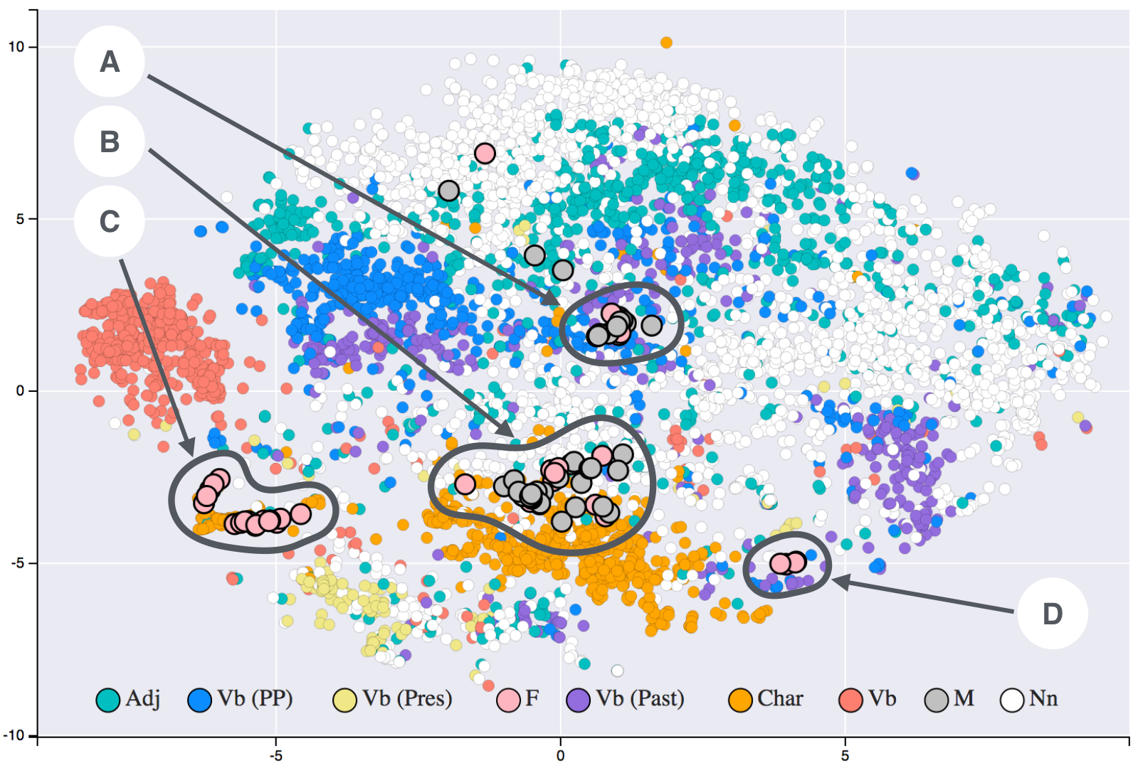
A picture like this is a little misleading in one way. The real space has hundreds of dimensions, and squashing it to two throws most of the structure away. Distances in the plot are hints, not measurements. Still, the clustering is real, and it came from nothing but which words showed up near which other words.

king - man + woman ≈ queen

Here is the result that made word vectors famous. In a 2013 NAACL paper, Mikolov, Yih and Zweig found that relationships between words show up as consistent offsets between their vectors. Take the vector for “king,” subtract “man,” add “woman,” and the result is very close to “queen.”⁷

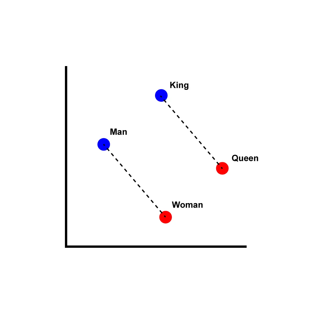
The way to read this is that there is roughly a “male to female” direction in the space. Moving along it turns “man” into “woman,” and “king” into something close to “queen.” The paper also tested grammar, with questions built from pairs like “see” and “saw” or “return” and “returned.” On that set of 8,000 syntactic analogy questions, the vectors got almost 40 percent right, which was a big deal at the time, and the same offset method beat the previous best systems on a SemEval semantic relations task.⁷

The method itself is short. You compute the target point, then search for the word whose vector is closest to it by cosine similarity:

def analogy(a, b, c, vectors, exclude_inputs=True):
    """a is to b as c is to ?   e.g. man : king :: woman : ?"""
    target = vectors[b] - vectors[a] + vectors[c]
    target /= np.linalg.norm(target)
    best, best_score = None, -1.0
    for word, v in vectors.items():
        if exclude_inputs and word in (a, b, c):
            continue                      # <- this line matters a lot
        score = v @ target / np.linalg.norm(v)
        if score > best_score:
            best, best_score = word, score
    return best

Look at the line marked “this line matters a lot.” That’s where the story gets more complicated.

When it fails

The standard analogy code, in word2vec’s own implementation, in the popular gensim library, and in other widely used code, never lets the answer be one of the three input words.⁸ That sounds like a harmless rule. Of course “king” isn’t the answer to “man is to king as woman is to what.”

Except it often would be. Nissim, van Noord and van der Goot reran the standard analogy test with that rule removed. Accuracy for the usual method dropped from 0.71 to 0.21.⁸ In most of the failures the answer was just the second input word. Ask “man is to king as woman is to ?” with the filter off, and the closest word is frequently “king” itself. The offset you added wasn’t big enough to move you off the starting word. The parallelogram is real in a loose sense, but the clean version depends on a search rule that quietly removes the most likely answer.

This matters beyond trivia. A widely cited 2016 paper by Bolukbasi and colleagues used analogies to show gender stereotypes in word vectors trained on Google News, with examples like “man is to computer programmer as woman is to homemaker.”⁹ The underlying finding, that these vectors encode stereotypes, holds up, and that paper’s own analysis didn’t rest only on analogies. But Nissim and colleagues showed that some of the most famous biased analogies are partly an artifact. With the input words allowed, “man is to doctor as woman is to ?” returns “doctor.”⁸ Under the original code, “doctor” could never come back, so the next closest word got reported instead. Their point was that the data is biased enough as is, and you don’t need to dramatize it.⁸

My takeaway is that the geometry of these spaces is approximate. Some relationships really do line up as directions. But “nearest word to a point” is a lossy question to ask of a 300-dimensional space, and the answer depends on choices you might not notice you made.

There’s a second, more basic failure. A static word vector gives “bank” exactly one point in space. The river sense and the money sense, plus “bank shot” and “you can bank on it,” all have to share it. The vector ends up somewhere in between, a blend of all the ways the word gets used. That is the problem the next step fixes.

Static vs. contextual: the residual stream

In a transformer, the embedding lookup is only the starting point. The row from the table goes into what’s called the residual stream: one vector per token position that flows up through the model. Each layer reads from the stream, computes something, and adds its result back in.

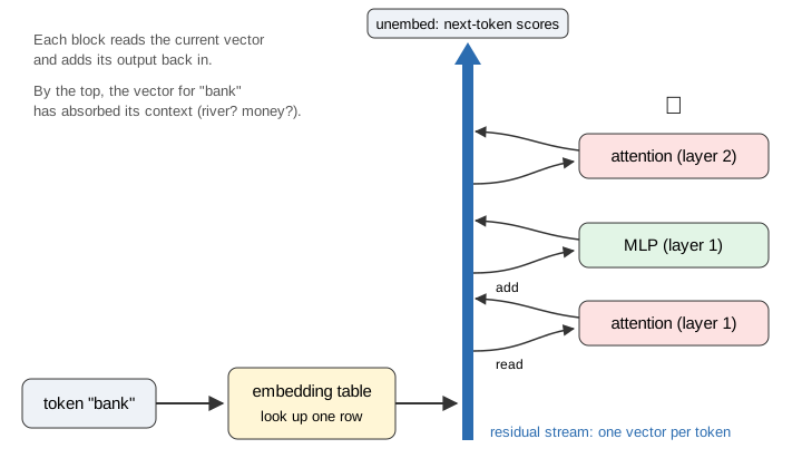
Anthropic’s interpretability team describes the residual stream as a communication channel: it doesn’t do any processing itself, and every layer communicates through it.¹⁰ Attention layers are how information moves between positions. If the sentence is “we sat on the bank and watched the river,” an attention layer can pull information from “river” into the vector at the “bank” position. Later layers then see a “bank” vector that has already been pushed toward the riverbank sense.

So there are two kinds of embeddings to keep apart:

• A static embedding is the row in the table. Same for “bank” in every sentence.
• A contextual embedding is the vector at that position after some layers. Different in every sentence.

How different? Kawin Ethayarajh measured this for ELMo, BERT and GPT-2 in 2019. A word’s vectors in different contexts are still more similar to each other than to other words’ vectors, but much less so in the upper layers. On average, less than 5 percent of the variance in a word’s contextual representations could be explained by a single static vector for that word.¹¹ By the middle of the model, the table row is a small part of what the vector holds.

He also found something odd: the contextual vectors weren’t spread evenly in every direction. They crowded into a narrow cone, in every layer of all three models.¹¹ That’s a hint that raw cosine similarity between hidden states can mislead you, since even unrelated words can look similar if everything points roughly the same way.

What does dimension 417 mean?

If the vector for a token has 768 numbers, you might expect number 417 to mean something, like a “plural” dimension or a “royalty” dimension.

Mostly no, for two reasons.

The first reason is that the residual stream doesn’t have what’s called a privileged basis. Every layer reads from it and writes to it through learned matrices. You could rotate the whole space, adjust every matrix that touches it to match, and the model would behave identically.¹⁰ If rotating the axes changes nothing, then the axes can’t carry special meaning. Dimension 417 is just an arbitrary coordinate in a space where directions matter and individual coordinates don’t.

You might hope it’s different for neurons, the places after a nonlinearity like ReLU, where individual units do have a special role. Sometimes it is. But often a single neuron responds to several unrelated things. In one small language model, Anthropic found a single neuron that responds to a mix of academic citations, English dialogue, HTTP requests and Korean text.¹² That’s called a polysemantic neuron.

The second reason explains why that happens. It’s called superposition.

More features than dimensions

Call a feature some property of the input the model cares about: “this is Python code,” “this is about the Golden Gate Bridge,” “this token is inside a quotation.” There are far more useful features in the world than there are dimensions in a model. If each feature needed its own axis, a 768-dimensional model could only track 768 things.

In “Toy Models of Superposition” (2022), Elhage and colleagues trained tiny networks to see what they do about this.¹³ In one setup they asked a model to store five features in just two dimensions. When the features were dense, meaning often active together, the model did the obvious thing: it kept the two most important features on their own axes and dropped the other three. When the features were sparse, meaning each one is rarely active, the model packed all five into the two dimensions, as directions spread around the circle.¹³

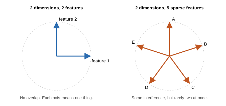
The trick works because of sparsity. If features A and B are almost never on at the same time, it doesn’t hurt much that their directions overlap a bit. The model pays a small cost in interference to represent way more things than it has room for. The authors describe the result as models that are, in some sense, noisily simulating a much larger network with no interference.¹³

This is the real answer to “what does dimension 417 mean.” In this picture, many features correspond to overlapping directions rather than separate axes. Any one coordinate is a mixture of pieces of many features. Looking at one number is like trying to understand a chord by listening to one frequency.

Sparse autoencoders: pulling the features back out

If features are directions packed in superposition, can we find them? That’s what sparse autoencoders, or SAEs, try to do.

The idea: train a second, much wider network to take a model’s activation vector, rewrite it as a combination of a large number of candidate directions, then rebuild the original vector from them. The catch is that only a few candidates are allowed to be active at once. That sparsity pressure pushes each candidate direction to line up with one feature instead of a blend.

In “Towards Monosemanticity” (2023), Bricken and colleagues did this on a one-layer transformer with a 512-neuron MLP layer.¹² They scaled the number of learned features from 512 up past 131,000. Many of the features were clean and specific in a way the neurons weren’t: one for Arabic script, one for DNA sequences, one for base64, one for Hebrew. The Hebrew feature was invisible in the neuron view entirely, since it wasn’t among the top activating examples for any single neuron.¹² They could also use features to steer the model: turning on the base64 feature made the model write base64, and turning on the Arabic feature made it write Arabic.¹² As they made the dictionary bigger, features split into families. One base64 feature in a small dictionary became three more specific ones in a larger dictionary.¹²

Then in May 2024, Templeton and colleagues scaled the same approach to Claude 3 Sonnet, a production model.¹⁴ They trained SAEs on the residual stream halfway through the model, with about 1 million, 4 million and 34 million features. Many features were abstract: the same feature would respond to a concept across languages, and even to images of it, though the SAE was trained only on text.¹⁴

The most famous one is a Golden Gate Bridge feature. Its strongest activations are almost all references to the bridge, and weaker ones include related landmarks and similar bridges.¹⁴ When they clamped that feature to ten times its maximum value during generation, the model started to identify itself as the Golden Gate Bridge.¹⁴

Honestly, that’s the result that made this click for me. A direction you found by looking at the model’s insides, turned up, changed what the model said about itself. That’s a causal test, which is much stronger evidence than a correlation.

I want to be careful about what this does and doesn’t show. SAE features are what the SAE found under its own sparsity pressure, and the papers themselves spend a lot of time on what fraction of the model’s behavior the features actually explain. A clean label on a feature is a hypothesis about it. The steering experiments are what make the hypothesis convincing.

So how does a word get meaning?

The surprising part is that nobody has to write down all the relationships we want the model to learn. Training gives it a reason to organize words in ways that help predict their context, and some of those relationships become visible when we look at the vectors.

That makes me wonder what else is in there that our favorite examples don’t reveal. An analogy that works is fun to inspect, but I’d also want to find the ones that fail and see how sensitive they are to the words we choose. The picture gets more interesting when we treat it as a way to explore what was learned, rather than a complete explanation of meaning.

Sources