What a neural network actually is, built up from one neuron

When I teach Python at Programming Club, a question that comes up is how “AI” works. Usually what they mean is: what is a neural network, physically, as in what numbers go where. I’ve spent a lot of this year looking at the hidden states of language models, and I still think the best way to answer is to start from one tiny piece and build up.

This post is my version of that build-up. The structure is inspired by 3Blue1Brown’s neural network series,¹ which is the best visual intro I know of and which uses the same running example I use here: reading handwritten digits. If you like this, go watch those. I’m writing my own version because explaining something is how I find out whether I actually get it.

The task: read a digit

Here is the problem. You get a small grayscale picture of a handwritten digit, and you have to say which digit it is, 0 through 9.

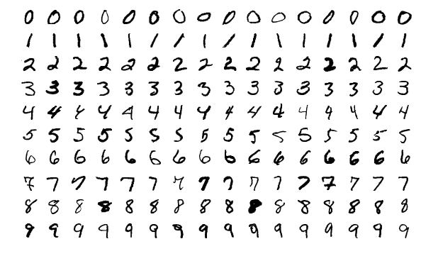
These come from MNIST, a dataset put together by Yann LeCun, Corinna Cortes and Chris Burges from older NIST handwriting collections. It has 60,000 training images and 10,000 test images. Each digit was scaled to fit in a 20 by 20 box and then centered in a 28 by 28 image.² It became the standard benchmark for this kind of thing after LeCun and colleagues used it in their 1998 paper on convolutional networks for document recognition.³

The thing that matters for us: a 28 by 28 image is 784 pixels, and each pixel is just a brightness. Call 0 black and 1 white. So the input to our network is a list of 784 numbers. The output should be 10 numbers, one per digit, where a bigger number means “I think it’s this one.” The whole network is a function that takes 784 numbers in and gives 10 numbers out.

That’s honestly it at the top level. Everything else is about what goes on inside that function.

One neuron

A neuron in a neural network is way simpler than the name suggests. It takes some numbers in, and gives one number out. Here is the recipe.

1. Multiply each input by its own weight.
2. Add those up.
3. Add one more number, the bias.
4. Pass the result through a squashing function.

Let’s do a tiny one with three inputs so you can see the arithmetic.

inputs:   x = [0.9, 0.0, 0.5]
weights:  w = [2.0, -1.0, 0.5]
bias:     b = -1.0

weighted sum = 2.0*0.9 + (-1.0)*0.0 + 0.5*0.5 = 1.8 + 0 + 0.25 = 2.05
plus bias    = 2.05 - 1.0 = 1.05

The weights decide what the neuron cares about. A big positive weight means “when this input is bright, push my output up.” A negative weight means “when this input is bright, push my output down.” The bias sets how easily the neuron turns on at all. With a bias of -1, the weighted sum has to get past 1 before this neuron gets excited.

Step 4 is the activation function; sigmoid is one example of a squashing function. The classic choice is the sigmoid, sigmoid(z) = 1 / (1 + e^(-z)). It takes any number and squishes it into the range 0 to 1. Very negative goes to about 0, very positive goes to about 1, and 0 goes to exactly 0.5.

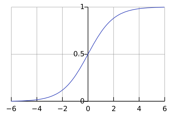
For our example, sigmoid(1.05) is about 0.74. So this neuron outputs 0.74. That number is called its activation.

Another common activation is ReLU, which is even simpler: relu(z) = max(0, z). Negative numbers become 0, positive numbers pass through unchanged. Nair and Hinton helped popularize it in 2010,⁴ and it tends to train better than sigmoid in deep networks because it doesn’t flatten out for large inputs. For this post I’ll mostly stick with sigmoid because “between 0 and 1” is easy to picture, but nothing important changes if you swap it.

This idea is old. Warren McCulloch and Walter Pitts described an artificial neuron in 1943 as a unit that fires when its weighted inputs cross a threshold, and showed that networks of these could compute logical functions.⁵ Their weights were set by hand. In 1958 Frank Rosenblatt’s perceptron added the part that makes it machine learning: a rule for adjusting the weights from examples.⁶

Layers, stacked into a network

One neuron looking at 784 pixels can only learn one pattern. A single neuron can, roughly, ask one question like “is there bright ink in this region and not in that one.” That isn’t enough to tell a 3 from an 8.

So you use many neurons at once. Each one looks at the same 784 inputs, but each has its own 784 weights and its own bias. If you have 16 of them, you get 16 outputs. That group is a layer.

The neurons in a layer don’t talk to each other. They all run in parallel on the same input, each asking its own question. The layer turns 784 numbers into 16 numbers.

Now take those 16 numbers and feed them into another layer of neurons. And then another. That is a neural network.

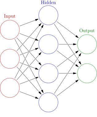
For digits, a classic small setup (the one 3Blue1Brown uses) is:¹

• Input layer: 784 numbers, the pixels. Not really neurons, just the data.
• Hidden layer 1: 16 neurons.
• Hidden layer 2: 16 neurons.
• Output layer: 10 neurons, one per digit.

“Hidden” just means “not the input and not the output.” The 16 is fairly arbitrary. You could use 100 and it would probably work better.

Let’s count the knobs. Layer 1 has 16 neurons, each with 784 weights and 1 bias, so 16 * 784 + 16 = 12,560. Layer 2 has 16 * 16 + 16 = 272. The output layer has 10 * 16 + 10 = 170. Total: 13,002 numbers. The network is that list of 13,002 numbers plus the recipe for using them. When people say a model has 7 billion parameters, they mean the same thing, just with a much longer list.

To read a digit, you set the 784 inputs to the pixel values, compute layer 1, use its outputs to compute layer 2, use those to compute the output layer, and look at which of the 10 outputs is biggest. That one-way trip is called a forward pass.

Why the squashing function matters so much

The squashing step looks like a detail. It is actually the whole reason stacking layers does anything.

Imagine you skip it. Then each layer just does “multiply by weights, add bias.” Try it with single numbers first.

layer A:  f(x) = 3x + 1
layer B:  g(y) = 2y - 5

stacked:  g(f(x)) = 2(3x + 1) - 5 = 6x - 3

Two layers, and the result is just another “multiply and add.” You could have used one layer with weight 6 and bias -3 and gotten the exact same function. Stack a hundred of them and it still collapses into one. Without the nonlinearity, a deep network is secretly a shallow one, and a shallow linear model can only draw straight-line boundaries between classes. That’s not enough for handwriting.

The squash breaks the collapse. Once each layer bends its output, layer B is working with something layer A could not have produced by itself, and stacking actually buys you something.

How much does it buy you? A lot, in theory. In 1989 George Cybenko proved that a network with just one hidden layer of sigmoid neurons can approximate any continuous function on a bounded region as closely as you want, if you give it enough neurons.⁷ Kurt Hornik, Maxwell Stinchcombe and Halbert White proved a similar result the same year for a much wider family of squashing functions.⁸ These are called the universal approximation theorems.

The catch, and the thing I wish more explanations said out loud: the theorem says a good set of weights exists. It doesn’t say how many neurons you need (it can be absurdly many), and it doesn’t say training will find those weights. It’s a statement about what is possible, not what is easy.

What the hidden layers might be doing

Here is the story everyone tells, and I like it as a starting point.

A digit is made of pieces. An 8 is two loops stacked. A 9 is a loop with a line under it. A 1 is mostly one vertical stroke. So maybe the first hidden layer learns to detect little edges and stroke fragments in different spots. The second hidden layer combines those into bigger parts, like “loop at the top” or “long vertical line.” Then the output layer combines parts into digits: loop on top plus line on the right means 9.

If that’s how it worked, each hidden neuron would have a clean job, and you could look at its weights and see an edge detector.

That’s a simplification, though, and probably more of a hope than a description. Nothing in training tells a neuron “you are the top loop detector.” Training only cares whether the final answer is right. When researchers look inside trained networks, they do find some neurons that respond to one clean, nameable feature. They also find lots of polysemantic neurons that respond to several unrelated things at once.⁹ One explanation is that networks pack more features into their neurons than they have neurons, smearing each feature across many of them, which an Anthropic paper studied under the name superposition.¹⁰ For a tiny 16-neuron digit network, my honest guess is that the hidden units look more like blurry mixtures than tidy edge detectors, and that the network gets the right answer anyway.

I still think the edges-then-loops story is the right way to start thinking about it. It’s a good intuition for why layers help. It’s just not a guarantee about what any specific network learned, and figuring out what networks actually learned is a whole research field. That’s the field I’ve been poking at lately.

Loss and training

So far the 13,002 weights could be anything. With random weights, the network outputs garbage. I’ll show that in code below. To make it good, we first need a way to measure how bad it is.

That measure is called the loss. It’s one number that says how wrong the network was on an example. Lower is better.

Concrete example. Say we show the network a 3. A common way to turn the 10 outputs into a guess is to rescale them so they add up to 1, like probabilities. Suppose after that, the network gives the digit 3 a probability of 0.6. A standard loss, called cross-entropy, is just the negative log of the probability the network gave the right answer:

loss = -ln(0.6) ≈ 0.51

Now suppose a worse network gives the right answer only 0.05:

loss = -ln(0.05) ≈ 3.00

And a network that knows nothing, spreading probability evenly over 10 digits, gives each one 0.1:

loss = -ln(0.1) ≈ 2.30

So the loss is near 0 when the network is confident and right, around 2.3 when it’s clueless, and climbs high when it’s confident and wrong. To judge the whole network, you average the loss over thousands of training images. 3Blue1Brown uses squared error instead (subtract what you wanted from what you got, square it, add up),¹ which works too. The idea is the same: one number for how wrong.

Training: nudge the weights downhill

Now the network has 13,002 knobs and one number, the average loss, that tells us how badly it’s doing. Training is the process of turning the knobs to make that number smaller.

Picture the loss as a landscape. Every possible setting of the 13,002 weights is a point, and the height at that point is the loss. You start somewhere random, which is usually high up. You want to walk downhill.

At any point, you can ask: if I nudge each weight a tiny bit, does the loss go up or down, and by how much? That collection of answers is the gradient. It points uphill, so you step the other way. Then you ask again and step again. That’s gradient descent. Do it many times over many training examples and the weights settle somewhere the loss is low, which means it fits the training examples better. Held-out images are how we check whether that carries over to new digits.

The hard part is computing the gradient efficiently. You need to know how each of 13,002 weights (or 7 billion) affects the loss, and doing that one weight at a time would be hopeless. The trick that makes it practical is backpropagation, made famous for neural networks by David Rumelhart, Geoffrey Hinton and Ronald Williams in 1986.¹¹ It works backward from the loss through the layers, reusing work as it goes. It deserves its own post, so I’m saving it for one.

The same thing, written with matrices

I’ve avoided matrices on purpose until now because I think they hide how simple each step is. But once you know what a layer does, the matrix version is just a compact way to write it.

Take layer 1. It has 16 neurons, each with 784 weights. Stack those weight lists as rows and you get a grid with 16 rows and 784 columns. Call it W. Put the 784 pixel values in a column x and the 16 biases in a column b. Then the whole layer is:

a = sigmoid(W x + b)

W x means: for each row of W, multiply it entry by entry with x and add up. That is exactly the weighted sum for one neuron, done for all 16 neurons at once. Adding b adds each neuron’s bias. sigmoid gets applied to each of the 16 numbers separately. Nothing new happened. It’s the same recipe from the one-neuron section, written in one line.

This also makes the collapse argument from earlier clean. Two layers with no squash give W2 (W1 x + b1) + b2, which multiplies out to (W2 W1) x + (W2 b1 + b2). That’s one matrix and one bias, so one layer. Same thing as 6x - 3, just bigger.

The other reason people use matrices is speed. GPUs are extremely good at multiplying big grids of numbers, so writing the network this way is what lets you run it fast.

One forward pass in NumPy

Here is the whole 784, 16, 16, 10 network doing one forward pass. The weights are random, so it hasn’t learned anything.

import numpy as np

rng = np.random.default_rng(0)
sizes = [784, 16, 16, 10]  # input, two hidden layers, output

# One weight matrix and one bias vector per layer, random for now (untrained)
Ws = [rng.normal(0, 0.1, (n_out, n_in)) for n_in, n_out in zip(sizes, sizes[1:])]
bs = [np.zeros(n_out) for n_out in sizes[1:]]

def sigmoid(z):
    return 1 / (1 + np.exp(-z))

x = rng.random(784)  # stand-in for a flattened 28x28 image, pixels in [0, 1]

a = x
for W, b in zip(Ws, bs):
    a = sigmoid(W @ a + b)  # every neuron in the layer: weighted sum, bias, squash

print("output activations:", np.round(a, 2))
print("network's guess:", a.argmax())
print("parameters:", sum(W.size + b.size for W, b in zip(Ws, bs)))

When I ran it, every output came out somewhere between 0.40 and 0.59, the “guess” was 8 for no good reason, and the parameter count printed 13002, which matches the hand count. The outputs come from random weights. They do not yet tell us anything useful about digits.

The loop in the middle is the entire forward pass. Two lines of real work.

From digits to language models

This is the part I find kind of wild. A large language model is the same idea, made much bigger and arranged more cleverly.

Instead of 784 pixels, the input is text chopped into tokens, each turned into a list of numbers. Instead of 16 neurons per hidden layer, there are thousands. Mistral 7B, one of the models I have been experimenting with, carries a list of 4,096 numbers for every token at every layer.¹² Instead of 13,002 parameters there are around 7 billion. There are extra parts, like attention, which lets each token look at the others. But inside every block of a transformer sits a small fully connected network built from learned linear maps and nonlinearities, often with gates and sometimes without biases. And training is still “measure how wrong, nudge the weights downhill.” The loss for a language model is the same cross-entropy from the loss section, applied to “how much probability did you give the actual next token.”

Those lists of numbers in the middle are hidden states, just like the activations in our small network. Making the model bigger gives it much more room to learn, but doesn’t automatically tell us how to describe what it learned.

That’s what makes me want to look more closely. We can follow the computation, yet still have questions about why a trained network responds the way it does. Training this small digit model and watching its hidden neurons change would be a way to start exploring that gap with something we can actually inspect.

Sources