Backpropagation as blame assignment

In my earlier post I built a neural network from one neuron up to a 784, 16, 16, 10 digit reader with 13,002 weights and biases. I ended on a promise. Training means nudging every one of those 13,002 numbers in the direction that lowers the loss, and to do that you need to know how each one affects the loss. The trick that makes that cheap is backpropagation, and I said it deserved its own post. This is that post.

The way I think about it: the network made a mistake, and backprop is the process of figuring out who is to blame for it, and by how much. Each weight gets a number that says “if you had been a little bigger, the loss would have changed this much.” That number is the weight’s share of the blame. Then every weight gets corrected in proportion to its share.

That sounds fancy. It’s honestly mostly bookkeeping. I’ll show that by doing the whole thing by hand on a network small enough to fit on one line.

Same notation as before

Quick recap, so the symbols match the last post. A neuron takes inputs, multiplies each by a weight w, adds a bias b, and squashes the result with the sigmoid:

z = w*x + b
a = sigmoid(z) = 1 / (1 + e^(-z))

I’ll call z the neuron’s raw sum and a its activation. The loss is cross-entropy: the negative log of the probability the network gave the right answer, loss = -ln(p_correct). Lower is better, 0 is perfect.

Training is gradient descent. For each weight, compute the slope of the loss with respect to that weight, written dL/dw, and step the other way:

w_new = w - learning_rate * dL/dw

So the entire job of backprop is to produce dL/dw for every weight. That’s it. It doesn’t update anything by itself. It just fills in the blame ledger.

The smallest network that still has a hidden layer

Here is the toy. One input, one hidden neuron, one output neuron. The output is a single sigmoid that means “probability this is the right class,” and for this example the right answer is yes, so the loss is -ln(a).

x  = 0.9                      (input, think of it as one bright pixel)
w1 = 2.0,  b1 = -1.0          (hidden neuron)
w2 = 1.0,  b2 = -0.5          (output neuron)

Forward pass

Work left to right, writing down every intermediate number. This part is exactly the forward pass from the last post.

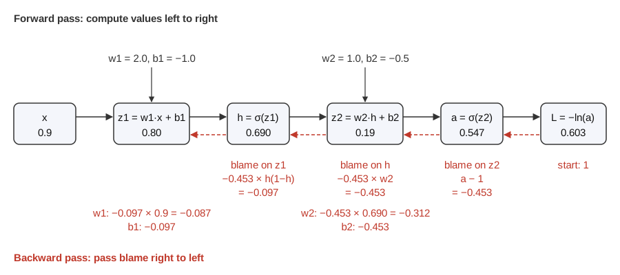
z1 = w1*x + b1  = 2.0*0.9 - 1.0  = 0.80
h  = sigmoid(0.80)               = 0.690
z2 = w2*h + b2  = 1.0*0.690 - 0.5 = 0.19
a  = sigmoid(0.19)               = 0.547
L  = -ln(0.547)                  = 0.603

The network gives the right answer a probability of 0.547. Barely better than a coin. The loss is 0.603. We want to know which of the four knobs, w1, b1, w2, b2, to turn and which way.

Backward pass

Now go right to left. At each step I ask one question: if this value went up a tiny bit, how much would the loss move? I’ll call that number the blame on that value. Formally it’s the partial derivative of the loss with respect to that value. Its sign tells you direction. Negative blame means “if I were bigger, the loss would go down,” so gradient descent will make it bigger.

Blame on z2. The loss is -ln(a) and a = sigmoid(z2). The slope of -ln(a) with respect to a is -1/a. The slope of the sigmoid has a famously clean form, a*(1 - a). Multiply them and almost everything cancels:

dL/dz2 = (-1/a) * a*(1 - a) = a - 1 = 0.547 - 1 = -0.453

I love this line. The blame at the output is just “what you said minus what was true.” You said 0.547, the truth was 1, you were short by 0.453. Sigmoid plus cross-entropy is a popular pairing partly because of this cancellation.

Blame on w2 and b2. z2 = w2*h + b2. If w2 goes up by a tiny amount, z2 goes up by h times that amount. So the blame on w2 is the blame on z2 times h. The bias feeds z2 with a slope of 1, so it gets the blame on z2 directly.

dL/dw2 = dL/dz2 * h = -0.453 * 0.690 = -0.312
dL/db2 = dL/dz2     = -0.453

Notice the pattern. A weight’s blame is the blame on the neuron it feeds, times the input it was multiplying. A weight that was multiplying something large had more influence, so it gets more blame. A weight multiplying zero gets none, which makes sense, since it couldn’t have changed anything.

Blame on h. Same equation, but now ask about the other input. h feeds z2 through w2, so:

dL/dh = dL/dz2 * w2 = -0.453 * 1.0 = -0.453

This is the step that makes it “back” propagation. The hidden neuron isn’t directly connected to the loss. It only matters through the output neuron, so it inherits blame from the output neuron, scaled by the weight connecting them.

Blame on z1. h = sigmoid(z1), and the sigmoid’s slope there is h*(1 - h) = 0.690 * 0.310 = 0.214.

dL/dz1 = dL/dh * h*(1 - h) = -0.453 * 0.214 = -0.097

Blame on w1 and b1. Same rule as for w2 and b2:

dL/dw1 = dL/dz1 * x = -0.097 * 0.9 = -0.087
dL/db1 = dL/dz1     = -0.097

Done. Here’s the whole thing in one picture.

Did it work?

Two checks. First, is the blame correct? The slow, obvious way to get the slope for one weight is to nudge it by a tiny amount, rerun the whole forward pass, and see how much the loss moved. I did that for all four knobs with a nudge of one millionth. The nudging gave -0.0871, -0.0968, -0.3123 and -0.4526, matching the backward pass to four decimal places.

Second, does following the blame actually help? Take one step with a learning rate of 1:

w1: 2.0  + 0.087 = 2.087
b1: -1.0 + 0.097 = -0.903
w2: 1.0  + 0.312 = 1.312
b2: -0.5 + 0.453 = -0.047

Rerun the forward pass with the new numbers, and the network now gives the right answer 0.712 instead of 0.547. The loss drops from 0.603 to 0.340. After 10 steps it’s at 0.054, and after 50 it’s at 0.011, with the network about 99% sure. (It’s only learning one example, so this is memorizing, but the mechanism is the same.)

Look at who changed most. b2 and w2 moved a lot, w1 and b1 barely moved. The output neuron was closest to the mistake, and blame got diluted on its way back through the hidden neuron’s sigmoid slope of 0.214. That dilution is a real thing. Stack enough sigmoids and the blame reaching the early layers gets multiplied by numbers no bigger than 0.25 again and again which can make it very small unless other factors, such as the weights along the path, compensate. That’s the vanishing gradient problem, and it’s a big part of why people moved to ReLU, whose slope is exactly 1 for positive inputs.¹

What I actually did there: the chain rule

Every step above was the same move. To find how the loss depends on something early, multiply the local slopes along the path from that thing to the loss:

dL/dw1 = dL/dz2 * dz2/dh * dh/dz1 * dz1/dw1
       = (a - 1) * w2 * h(1 - h) * x

That’s the chain rule from calculus. Backprop is the chain rule with one specific discipline: start at the loss and work backward, saving each intermediate blame so you can reuse it.

The reuse is the whole point. dL/dz2 got computed once and then used three times: for w2, for b2, and to pass back to h. dL/dz1 got computed once and used twice. In a real network, the blame on one hidden neuron gets reused for every one of the hundreds of weights feeding into it. Nobody ever recomputes a path from scratch.

Computational graphs

The picture above is a computational graph. Each box is one value, and each arrow means “this value was computed from that one.” Every program that computes a number can be drawn this way, not just neural networks. Once it’s a graph, backprop is a mechanical rule you can apply to any graph:

1. Run forward, saving every value.
2. Set the blame on the final output to 1 (the loss changes one-for-one with itself).
3. Visit the nodes in reverse order. Each node takes the blame it received, multiplies by the local slope of each of its inputs, and sends that to those inputs.

Chris Olah’s post on this is the clearest one I’ve read.² One thing it points out that my toy didn’t show: what happens when a value is used in more than one place.

When a value feeds two places, blame adds

In the toy network every value fed exactly one thing. In the real digit network, each pixel feeds all 16 neurons in the first hidden layer, and each hidden neuron feeds every neuron in the next layer. So what’s the blame on a value with several outgoing arrows?

You add them up. Here’s a tiny example. Say y = x*x + 3*x at x = 2, so y = 10. Draw x as one node with three outgoing arrows: two into the multiply and one into the 3*x.

via first factor of x*x:   slope is the other factor = 2
via second factor of x*x:  slope is the other factor = 2
via 3*x:                   slope is 3

total blame on x = 2 + 2 + 3 = 7

And from calculus, dy/dx = 2x + 3 = 7. Same answer. That’s the multivariable chain rule: if x affects the output through several paths, the total effect is the sum of the effects along each path. Olah’s post frames it exactly that way, as summing over paths, and points out that summing over every path explicitly blows up combinatorially in a deep network.² Backprop avoids that by merging the blame at each node before passing it on, so each edge gets visited once.

In the code below, that “add up the blame from everything you feed” step is a single matrix multiply.

Scaling up to the digit network

Here’s the 784, 16, 16, 10 network from last time, now with a backward pass. The output layer uses softmax, which is the “rescale the 10 outputs so they add up to 1” step I mentioned in the loss section of the last post, and the loss is cross-entropy. That pairing has the same nice cancellation as sigmoid with one output: the blame on the output layer’s raw sums is “your probabilities minus the one-hot truth.”

import numpy as np

rng = np.random.default_rng(0)
sizes = [784, 16, 16, 10]
Ws = [rng.normal(0, 0.1, (n_out, n_in)) for n_in, n_out in zip(sizes, sizes[1:])]
bs = [np.zeros(n_out) for n_out in sizes[1:]]

def sigmoid(z):
    return 1 / (1 + np.exp(-z))

def softmax(z):
    e = np.exp(z - z.max())
    return e / e.sum()

def loss_and_grads(x, label):
    # forward pass, remembering every layer's activation
    acts = [x]
    for W, b in zip(Ws[:-1], bs[:-1]):
        acts.append(sigmoid(W @ acts[-1] + b))
    p = softmax(Ws[-1] @ acts[-1] + bs[-1])
    loss = -np.log(p[label])

    # backward pass: blame on the output layer's z is "what you said minus the truth"
    dz = p.copy()
    dz[label] -= 1
    dWs, dbs = [], []
    for i in reversed(range(len(Ws))):
        dWs.insert(0, np.outer(dz, acts[i]))  # blame on each weight = blame on its neuron * input it saw
        dbs.insert(0, dz)
        if i > 0:
            da = Ws[i].T @ dz                  # send blame back along the same weights
            dz = da * acts[i] * (1 - acts[i])  # through the sigmoid's slope
    return loss, dWs, dbs

Every line in the backward loop is one of the steps from the hand calculation, just done for a whole layer at once.

• np.outer(dz, acts[i]) is “blame on the neuron times the input it saw,” for every weight in the layer. That’s dL/dw2 = dL/dz2 * h, 12,544 times for the first layer.
• dbs gets dz directly, same as dL/db2 = dL/dz2.
• Ws[i].T @ dz is “send blame back through the weights.” The transpose is what does the adding-up from the previous section. Row j of W.T holds every weight leaving neuron j, so the multiply sums the blame from all the neurons it feeds.
• acts[i] * (1 - acts[i]) is the sigmoid slope, h*(1 - h).

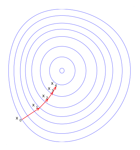
I checked one weight the slow way, same as before. For the weight connecting pixel 400 to hidden neuron 5, backprop said 1.31337e-05 and nudging said 1.31337e-05, agreeing to about six significant figures. Then I ran five steps of gradient descent on that single fake image with a learning rate of 0.5, and the loss went 2.136, 0.590, 0.201, 0.115, 0.079.

Why backward and not forward

This is the part that shows backprop is an efficiency trick, not a learning rule.

Remember the slow way, nudging one weight and rerunning? It works. My gradient checks used it. The problem is it costs one extra forward pass per weight. For the digit network that’s 13,002 forward passes to get one gradient. For a 7 billion parameter model it’s 7 billion forward passes, for one step.

There’s also a smarter version that goes in the forward direction, called forward-mode differentiation. It carries “how much does everything depend on this one input” along with the values as they’re computed, and it’s exact rather than approximate. But it still needs one pass per input you care about. The Baydin et al. survey puts it plainly: for a function from n inputs to one output, forward mode needs n evaluations to build the gradient.³

Backprop is reverse-mode differentiation. It flips the direction: one backward pass gives the blame on every input at once, because it starts from the single output and fans out. The cost of that backward pass is a small constant multiple of the forward pass. The survey, citing Griewank and Walther, gives that constant as guaranteed under 6 and typically around 2 to 3.³ So a full gradient for all 13,002 weights costs roughly the same as two or three forward passes instead of 13,002. Neural network training is the extreme version of “many inputs, one output”: millions or billions of weights, one loss number. That’s exactly the shape where reverse mode wins.

The price is memory. To run backward, you need the values from the forward pass (h and a in the toy, acts in the code). That’s why training a big model takes way more memory than running it.

Autodiff: letting a framework handle the backward pass

I wrote the backward loop by hand above because I wanted to see every step. For most model code, frameworks do this for you with automatic differentiation, or autodiff.

Baydin, Pearlmutter, Radul and Siskind’s survey is the reference I’d point to. They describe autodiff as a family of techniques more general than backpropagation for computing exact derivatives of functions written as computer programs, and they describe backprop as just a special case: reverse mode autodiff applied to a network’s loss as a function of its weights.³ They also lay out why the two obvious alternatives don’t work for this. Numerical differentiation (my nudging trick) has rounding and truncation error and scales badly with the number of weights. Symbolic differentiation (the kind a computer algebra system does) gives exact formulas but suffers from “expression swell,” where the derivative expression gets enormous.³

PyTorch’s autograd is a working version of the graph idea. As the forward pass runs, it records every operation into a directed acyclic graph, with your input tensors as leaves and the output as the root. When you call .backward() on the loss, it walks that graph from the root back to the leaves, applies the chain rule at each node, and accumulates the results in each tensor’s .grad. The graph gets rebuilt from scratch every iteration, which is why you can use normal Python if statements and loops in a model.⁴ The “accumulates” part is the blame-adds-up rule from earlier.

If you want to see how little code that actually takes, Andrej Karpathy’s micrograd is a scalar autograd engine in about 100 lines, plus a tiny neural network library in about 50, and it’s enough to train small networks.⁵ Each value object remembers its parents and how to pass blame back to them. That’s the whole engine.

I read through micrograd while writing this, and I think rebuilding it from scratch is the next thing I’d try, because it would force me to write the local slope for every operation myself.

Who came up with this

The 1986 paper that made backprop famous in machine learning is Rumelhart, Hinton and Williams in Nature.⁶ Their framing is the same as this post’s: repeatedly adjust the weights to shrink the gap between the network’s actual output and the desired output. Their big claim was what that does to the hidden units. Through those adjustments, the hidden units, which are neither input nor output, come to represent important features of the task. That’s the hope I talked about last time with edge detectors and loops.

But they weren’t the first to find the math, and the history is messy in a way I find kind of reassuring. The Baydin survey says Seppo Linnainmaa’s 1970 and 1976 work is often cited as the first published description of reverse mode, and that Paul Werbos cast it in more formal, step-by-step terms in his 1974 PhD thesis.³⁷ Andreas Griewank wrote a whole history paper on the question of who invented it and concluded there’s no single answer: versions came up from the late 1960s on, in different fields that weren’t talking to each other.⁸ He also tells the story that Linnainmaa said the idea came to him in a park in Copenhagen in 1970, while he was working on how rounding errors build up in a calculation.⁸ Baydin et al. note that the machine learning community reinvented it more than once, and that the 1986 group only learned about some of the earlier work after their own discovery.³

What backprop doesn’t do, and what’s next

Backpropagation gives us gradients. The optimizer decides how to use them to change the weights. Neither step tells us in advance what a trained network will learn to represent.

That’s the part I find surprising. We can follow every operation in this example, yet knowing the procedure doesn’t give us a clear picture of the network we’ll end up with. I’d like to train the small digit model and inspect its hidden neurons as it learns. Do recognizable features appear, or does it find a way of solving the task that is harder for us to describe? Even a small network leaves room for that kind of discovery.

Sources