Say you have three piles of sand in a row and three holes a little further down the road. You want to fill the holes with the sand. Every bucket you carry costs effort, and carrying it further costs more. What is the cheapest way to do it?
That question goes back to 1781, it is tied to a Nobel Prize, and it shows up all over machine learning now. I used a version of it in a project I ran this summer to compare groups of a language model’s hidden states.
I could run the code, but I couldn’t have explained to you why it worked. So this post is me fixing that. We will start with sand, get to a precise definition, see when its use of geometry helps, and end with an algorithm you can write in a few lines.
The sand problem
Here is a concrete version. All positions are in meters along a straight road.
| Pile | Position | Buckets |
|---|---|---|
| A | 0 | 3 |
| B | 1 | 2 |
| C | 2 | 1 |
| Hole | Position | Buckets needed |
|---|---|---|
| X | 1 | 1 |
| Y | 3 | 2 |
| Z | 4 | 3 |
Six buckets of sand, six buckets of hole. The sand has to go somewhere, and every hole has to end up full.
For the cost of moving one bucket, I will use the squared distance. Moving a bucket 1 meter costs 1, moving it 2 meters costs 4, moving it 4 meters costs 16. Squaring punishes long trips a lot, which roughly matches how annoying it is to carry sand far. (You could use plain distance too, but with plain distance on a line this example has a lot of tied best plans, and the exact solver can hand back a plan that looks nothing like the “keep things in order” one and still costs the same. Squared cost gives a single clear winner.)
So the cost of moving one bucket from each pile to each hole is a little table:
        X(1)  Y(3)  Z(4)
A(0)      1     9    16
B(1)      0     4     9
C(2)      1     1     4
A plan is just a table of the same shape that says how many buckets go from each pile to each hole. The rows have to add up to what each pile has, and the columns have to add up to what each hole needs. The total cost is each entry of the plan times the matching entry of the cost table, all added up.
If you try a few plans by hand you start to notice something. Sending pile A’s stuff to Z is expensive, because A is the farthest left and Z is the farthest right. The cheap plans keep things in order: leftmost sand fills leftmost holes. The best plan turns out to be:
        X  Y  Z
A       1  2  0
B       0  0  2
C       0  0  1
Total cost: 1*1 + 2*9 + 2*9 + 1*4 = 41. I checked this with an exact solver from the POT library, which is the standard Python optimal transport toolkit.1 That number, the minimum total cost of turning one pile shape into another, is the whole idea of optimal transport.
Monge’s version and Kantorovich’s fix
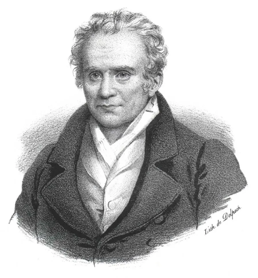
The problem really did start with dirt. In 1781 Gaspard Monge presented a memoir to the French Academy of Sciences about how to move soil from an excavation into a fill at the least cost.2
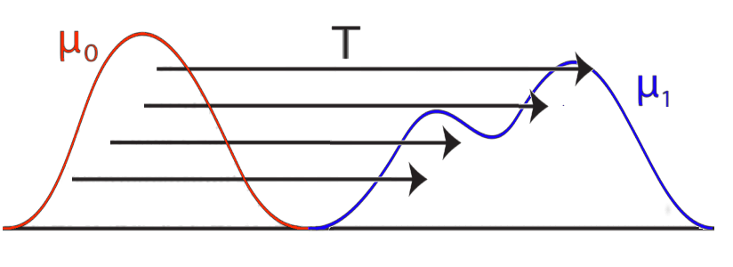
Monge’s version had a restriction that made it really hard. Each grain of sand had to go to exactly one place. You pick a map T that sends every point in the pile to one point in the hole, and you can’t split anything.
That breaks immediately in simple cases. If the source is one pile of 2 buckets and the target is two holes of 1 bucket each, there is no valid map, because the single pile has to go to one place. You need to split it.
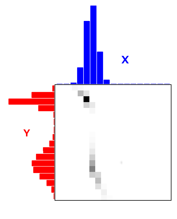
In 1942 Leonid Kantorovich wrote a short paper that relaxed the problem.3 Instead of a map, you choose a plan: a table (or in the continuous case, a joint distribution) that says how much mass goes from each source point to each target point. Mass can be split. That is exactly the table I wrote above. The constraints become “rows sum to the source, columns sum to the target,” and the cost is linear in the plan, so the whole thing is a linear program.
This turned out to matter well outside math. Kantorovich shared the 1975 Nobel Prize in economics with Tjalling Koopmans for their work on the optimal allocation of resources.4 Moving sand and moving supplies between factories are the same problem.
From sand to distributions
Here is the jump that makes this useful for ML. Divide every pile by the total, so the piles add up to 1. Now the sand is a probability distribution and the holes are another one. The minimum cost measures how much transport is needed; the precise distance depends on the cost and any root taken afterward.
With squared distance as the cost, you take the square root of the minimum cost and call it the 2-Wasserstein distance. With plain distance as the cost, it is the 1-Wasserstein distance, which people also call the earth mover’s distance. The name stuck in computer vision. Rubner, Tomasi, and Guibas used it in 2000 to compare color histograms of images for image search, and showed that for distributions with the same total mass it is a true metric.5
Why not just use KL divergence?
If you’ve trained a model, the distance between distributions you probably know is KL divergence. Cross-entropy loss is KL plus a constant. So why bother with any of this?
KL compares the two distributions point by point. For each place, it asks how much probability P puts there versus how much Q puts there:
KL(P || Q) = sum over x of P(x) * log( P(x) / Q(x) )Notice what is missing: any idea of how far apart two places are. KL has no ruler. Position 3 and position 3.01 are as unrelated to it as position 3 and position 3,000.
That causes a very specific failure. Take two spikes of sand, one at position 0 and one at position s. If s is anything other than 0, the first distribution puts mass where the second has zero, so log(P(x)/0) blows up and the KL is infinite. Move the spike from 1 meter away to 1,000 meters away and KL says the same thing: infinite. The symmetric version, Jensen-Shannon, is stuck at a constant log 2 for any nonzero shift.
The Wasserstein distance for the same setup is just |s|. Move the spike closer and the distance goes down smoothly. This exact example is in the Wasserstein GAN paper by Arjovsky, Chintala, and Bottou (2017), and it is a key part of their argument.6 If you are training a generator and its outputs don’t overlap the real data yet, which is normal early in training, KL and JS give you no useful gradient. Nothing tells the model “you’re getting warmer.” Wasserstein does.
This is the part that matters most to me. A loss function is a way of telling a model which direction is better. If the distance can’t tell “close” from “far” when the supports don’t overlap, it can’t point anywhere. Optimal transport bakes the geometry of the space into the distance, so “closer” actually means closer.
The catch, and Sinkhorn’s fix
So why isn’t everyone using Wasserstein for everything? Cost.
Solving the linear program exactly for two distributions with n points each takes roughly cubic time in n. Marco Cuturi’s 2013 paper points out that this gets costly once the histograms have a few hundred bins.7 If you want to compute it inside a training loop, on a batch, on every step, that’s a problem. It also doesn’t map nicely onto a GPU, which wants big batched matrix multiplies and not a combinatorial solver.
Sinkhorn: blur the plan a little
Cuturi’s fix is the thing this post is named after. Add a small reward for plans that are spread out.
Formally, you add an entropy term to the cost:
minimize   sum(P * C)  -  eps * H(P)
where      H(P) = -sum(P * log P)
subject to rows of P sum to a, columns sum to b
eps is a knob. When it’s big, the solver prefers spreading every pile across every hole a bit. When it’s small, you get close to the exact sharp plan. Cuturi calls the result the Sinkhorn distance, and the abstract says it can be computed several orders of magnitude faster than standard transport solvers.7
The surprising part is what the solution looks like. With the entropy term, the optimal plan always has this form:
P = diag(u) @ K @ diag(v) where K = exp(-C / eps)K is fixed. It is just the cost table turned into weights, with cheap moves getting big weights and expensive moves getting tiny ones. All you have to find are two vectors, u (one number per pile) and v (one number per hole), that rescale the rows and columns of K until the rows add up to the piles and the columns add up to the holes.
And there’s an old, simple way to do that. Fix the rows. Then fix the columns. Fixing the columns messes the rows up a little, so fix the rows again. Repeat. Richard Sinkhorn proved in 1964 that for any matrix with all positive entries, this alternating rescaling converges to a matrix whose rows and columns have the sums you want.8 That is why it’s called Sinkhorn, and it’s why the trick works: K is all positive because exp of anything is positive.
The algorithm in a few lines
Here it is in NumPy, run on the sand example.
import numpy as np

def sinkhorn(a, b, C, eps=0.3, iters=2000):
    K = np.exp(-C / eps)              # cheap moves get big weights
    u = np.ones_like(a)
    for _ in range(iters):
        v = b / (K.T @ u)             # rescale so columns hit the holes
        u = a / (K @ v)               # rescale so rows hit the piles
    P = u[:, None] * K * v[None, :]   # the transport plan
    return P, np.sum(P * C)

x = np.array([0., 1., 2.]); a = np.array([3., 2., 1.]) / 6   # piles
y = np.array([1., 3., 4.]); b = np.array([1., 2., 3.]) / 6   # holes
C = (x[:, None] - y[None, :]) ** 2
P, cost = sinkhorn(a, b, C)
That’s it. Every step is a matrix-vector product and an elementwise divide, which is exactly what GPUs are good at, and it’s differentiable, so you can backprop through it.
I ran it at a few values of eps and scaled the answer back up to buckets so it matches the table from earlier. The exact answer is 41.
| eps | Sinkhorn cost | What the plan looks like |
|---|---|---|
| 10 | 46.27 | Every pile sends a bit to every hole. Very blurry. |
| 1 | 42.24 | Mostly the right shape, with some leaking. |
| 0.3 | 41.14 | Almost exact. A few tenths of a bucket in the wrong spot. |
At eps = 0.3 the plan came out as:
        X     Y     Z
A     1.00  1.93  0.07
B     0.00  0.07  1.93
C     0.00  0.00  1.00
You can see the exact plan underneath, slightly smeared. That smear is the price of speed.
Things that will bite you
A few practical notes, from running this and from reading around.
Small eps makes convergence and numerical stability harder. At eps = 0.1, the largest cost gives the smallest kernel entry, exp(-16 / 0.1), about 3.3e-70. That is representable in float64, so it is not itself underflow. The simple iteration can converge slowly; at still smaller eps, entries can underflow to zero and scaling can fail. The standard fix is to do the whole thing in log space with log-sum-exp. Peyré and Cuturi’s book covers this and a lot more.9 In practice, just use POT or a library that already does it.1
Sinkhorn distance of a thing to itself isn’t zero. Because of the blur, comparing a distribution to itself gives a small positive number. Feydy and coauthors fixed this with the Sinkhorn divergence, which subtracts off the self-comparison terms. Their paper also shows that as eps goes from 0 to infinity, it slides from true optimal transport over to a simpler kernel distance called MMD.10 So eps is a dial between “respects geometry fully” and “cheap and smooth.”
You have to pick a cost. Everything above depends on C. On a road, distance is obvious. For images, words, or hidden states, choosing what “far” means is the actual modeling decision, and OT can’t make it for you.
Where it shows up
Wasserstein GANs
Already mentioned, but worth saying what they did. The WGAN paper doesn’t run Sinkhorn. It uses a different (dual) way of writing the 1-Wasserstein distance, where a second network, the critic, learns a function whose slope is limited, and the distance becomes the gap between the critic’s average score on real data and on fake data.6 The motivation is the spike example: they wanted a loss that keeps giving a useful signal even when real and generated data barely overlap.
Word mover’s distance
This one I like a lot because it’s so literal. Kusner and coauthors in 2015 asked: how different are two documents? Their answer: turn every word into a word embedding, so each document becomes a cloud of points, and then compute the minimum cost of moving one cloud onto the other.11 Their own example: “Obama speaks to the media in Illinois” and “The President greets the press in Chicago” share almost no words, but “Obama” is close to “President” and “Illinois” is close to “Chicago” in embedding space, so the move is cheap. They showed it beat the baselines they tested for nearest-neighbor document classification on eight datasets.
If you want the background on where those word vectors come from and why distances between them mean anything, I wrote about that in how a word gets meaning inside a model.
Comparing sets of hidden states
This is how I ended up here. A language model writing text produces one hidden-state vector per token. If you want to compare “what the model was doing in these 10 tokens” to “what it’s doing in these 10 tokens,” you have two small clouds of vectors. You could average each cloud and compare the averages, but that throws away the shape. Optimal transport compares the clouds as clouds: match up states one to one (or fractionally), pay for the distance each one moves, and add it up.
That’s what I used a Sinkhorn distance for in a project this summer, comparing groups of hidden states from a model as it worked through math problems. I’ll write about that project properly another time. For this post, the useful part is the question Sinkhorn actually answers: how much work does it take to rearrange this set of states into that one. Thinking of it as piles of sand made it a lot clearer to me what my code was measuring, and what it couldn’t.
What I’d want you to take away
What I like about transport is that it makes us choose what moving between two things should cost. That choice carries an idea of similarity, and it can change the answer even when the piles themselves stay the same.
I’d like to explore that by changing the cost and the amount of smoothing in the same small example. When does a broad match reveal a useful pattern, and when does it hide a difference we care about? Seeing those changes would help me understand when transport is worth using, beyond being an elegant way to compare two distributions.
Sources
Footnotes
-
R. Flamary et al., “POT: Python Optimal Transport”, Journal of Machine Learning Research 22(78), 2021, https://pythonot.github.io/ ↩ ↩2
-
Bibliothèque nationale de France, “Des tas de sable aux pixels, deux siècles et demi de transport optimal depuis Monge” (on G. Monge, “Mémoire sur la théorie des déblais et des remblais”, Histoire de l’Académie Royale des Sciences, 1781, pp. 666-704), https://www.bnf.fr/fr/mediatheque/des-tas-de-sable-aux-pixels-deux-siecles-et-demi-de-transport-optimal-depuis-monge ↩
-
L. Kantorovich, “On the translocation of masses”, Doklady Akademii Nauk SSSR 37, 1942. English translation in Management Science 5(1), 1958, https://www.math.utoronto.ca/mccann/assignments/477/Kantorovich42.pdf ↩
-
NobelPrize.org, “The Sveriges Riksbank Prize in Economic Sciences in Memory of Alfred Nobel 1975”, https://www.nobelprize.org/prizes/economic-sciences/1975/summary/ ↩
-
Y. Rubner, C. Tomasi, L. J. Guibas, “The Earth Mover’s Distance as a Metric for Image Retrieval”, International Journal of Computer Vision 40(2), 2000, https://people.eecs.berkeley.edu/~efros/courses/LBMV07/Papers/rubner-jcviu-00.pdf ↩
-
M. Arjovsky, S. Chintala, L. Bottou, “Wasserstein GAN”, arXiv, 2017, https://arxiv.org/abs/1701.07875 ↩ ↩2
-
M. Cuturi, “Sinkhorn Distances: Lightspeed Computation of Optimal Transport”, NeurIPS 2013, https://arxiv.org/abs/1306.0895 ↩ ↩2
-
R. Sinkhorn, “A Relationship Between Arbitrary Positive Matrices and Doubly Stochastic Matrices”, Annals of Mathematical Statistics 35(2), 1964, https://doi.org/10.1214/aoms/1177703591 ↩
-
G. Peyré, M. Cuturi, “Computational Optimal Transport”, Foundations and Trends in Machine Learning 11(5-6), 2019, https://arxiv.org/abs/1803.00567 ↩
-
J. Feydy, T. Séjourné, F.-X. Vialard, S. Amari, A. Trouvé, G. Peyré, “Interpolating between Optimal Transport and MMD using Sinkhorn Divergences”, AISTATS 2019, https://arxiv.org/abs/1810.08278 ↩
-
M. Kusner, Y. Sun, N. Kolkin, K. Weinberger, “From Word Embeddings To Document Distances”, ICML 2015, https://proceedings.mlr.press/v37/kusnerb15.html ↩