If you read anything about language models, you run into this line sooner or later:
Attention(Q, K, V) = softmax(Q K^T / sqrt(d_k)) VIt comes from the 2017 Transformer paper, “Attention Is All You Need”.1 It looks like the kind of formula you nod at and move past. It is also small enough to do by hand. Four words, vectors with two numbers each, and some arithmetic you could do on the back of a worksheet.
That is what this post is. I am going to run attention on one tiny sentence, number by number, draw what happens, and then zoom out to what it means and what it does not mean. I wrote about the paper itself a few weeks ago in Attention Is All You Need, read in 2026. This one is the mechanics.
The first time I tried to understand attention I only got it once I did the numbers on paper, so that is how I am going to walk through it here.
The problem attention solves
Take the sentence “the cat sat down”. By the time a model processes the word “sat”, it would help a lot to know who did the sitting. The vector for “sat” on its own, the one that comes out of the embedding table, knows nothing about cats. It is the same vector in “the dog sat” and “the committee sat”. (I wrote about where those starting vectors come from in How a word gets meaning inside a model.)
So each word needs a way to pull in information from the other words. The catch is that which words matter changes every time. In “the cat sat down”, “sat” wants “cat”. In “she said the cat sat down”, the word “said” probably cares more about “she”. You cannot hard-wire it.
The idea predates the Transformer. In 2014, Bahdanau, Cho and Bengio were working on translation with recurrent networks, which squeezed the whole source sentence into a single fixed-length vector before translating. They called that fixed vector a bottleneck and let the model do a soft search over the source words for each output word instead.2 That soft search is attention. The 2017 paper’s move was to drop the recurrence and build the whole network out of attention plus small feed-forward layers.1
Three roles for every word
Here is the core picture. Every word in the sentence plays three roles at once.
- A query: what am I looking for?
- A key: what do I contain, as a label other words can match against?
- A value: if someone decides I am relevant, what information do I hand over?
Each one is a vector, and each one is made from the word’s current vector by multiplying it by a learned matrix: q = x @ W_Q, k = x @ W_K, v = x @ W_V. The model learns those three matrices during training. Nobody tells it what a “query” should mean. It just finds matrices that make the predictions better.
Jay Alammar’s Illustrated Transformer is where a lot of people first saw this laid out visually, and it is worth reading alongside this.3 What I want to add is the actual arithmetic.
For our toy, I am going to skip the matrix multiplication and just pick the query, key and value vectors directly, two numbers each. In a real model these would come out of learned weights and have dozens or hundreds of dimensions. Two is enough to see everything.
| word | query q | key k | value v |
|---|---|---|---|
| the | [0, 1] | [0, 1] | [1, 0] |
| cat | [1, 1] | [2, 0] | [4, 0] |
| sat | [2, 0] | [1, 1] | [0, 2] |
| down | [1, 0] | [0, 2] | [1, 1] |
I picked these so that the query for “sat” points the same direction as the key for “cat”. You can read that as “sat” asking “who is the subject here?” and “cat” carrying a key that says “I am a noun that could be a subject”. That story is mine, not the model’s. Real learned directions are rarely that clean. But it makes the numbers easy to follow.
Doing it by hand
Step 1: score every word
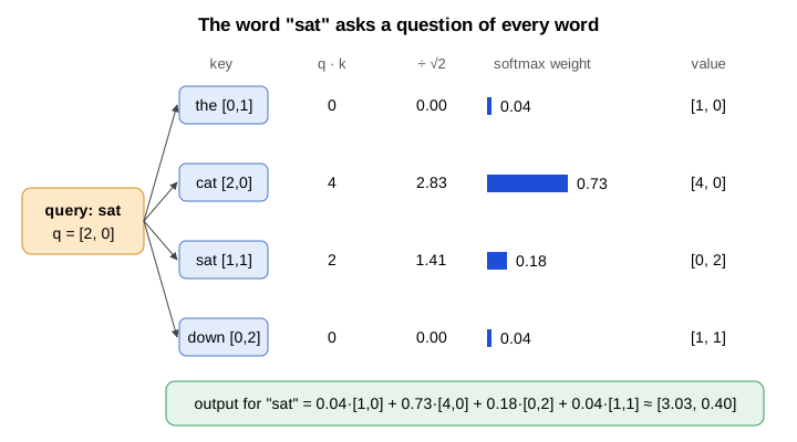
We will compute the output for one word, “sat”. Its query is q = [2, 0].
The score between “sat” and each word is a dot product: multiply matching entries and add. A dot product grows when vectors align and when their lengths grow; it is zero when they are at right angles.
sat . the  = 2*0 + 0*1 = 0
sat . cat  = 2*2 + 0*0 = 4
sat . sat  = 2*1 + 0*1 = 2
sat . down = 2*0 + 0*2 = 0
So the raw scores are [0, 4, 2, 0]. “cat” matches best, “sat” matches itself a little, and “the” and “down” do not match at all.
Step 2: scale
Next we divide by sqrt(d_k), where d_k is the length of the key vectors. Here d_k = 2, so we divide by about 1.414.
[0, 4, 2, 0] / 1.414 = [0.00, 2.83, 1.41, 0.00]This step looks like housekeeping, and it kind of is, but it matters. The dot product of two vectors with many entries is a sum of many terms, so it tends to grow as the vectors get longer. The paper’s authors suspected that large dot products push the softmax (next step) into a region where its gradients become extremely small, which makes training stall, and the division is there to counteract that.1
You can see the effect without any calculus. Here is softmax on our raw scores, and then on the same scores times ten, which is roughly what happens when vectors get long:
softmax([0, 4, 2, 0])    = [0.02, 0.85, 0.12, 0.02]
softmax([0, 40, 20, 0])  = [0.00, 1.00, 0.00, 0.00]
The second one has stopped being a soft choice. It is a hard pick, and a hard pick barely changes when you nudge the inputs, so learning has nothing to push on. Scaling keeps the scores in a range where the model can still change its mind.
Step 3: softmax
Softmax turns any list of numbers into positive weights that add up to 1. Raise e to each number, then divide each result by the total.
exp(0.00) = 1.00
exp(2.83) = 16.92
exp(1.41) = 4.11
exp(0.00) = 1.00
total     = 23.03

weights = [1.00, 16.92, 4.11, 1.00] / 23.03
        = [0.04, 0.73, 0.18, 0.04]
(The rounded weights add to 0.99. The unrounded ones add to exactly 1.)
So “sat” puts 73 percent of its attention on “cat”, 18 percent on itself, and a little on the other two. With finite scores, softmax gives every unmasked position positive weight, though that weight can be tiny. The causal mask below deliberately makes some weights zero.
Step 4: take the weighted average of the values
Now the keys and queries are done. They only decided the weights. The information that actually moves comes from the values.
output(sat) = 0.04*[1,0] + 0.73*[4,0] + 0.18*[0,2] + 0.04*[1,1]
            = [3.03, 0.40]
(That uses the unrounded weights. With the rounded ones shown you get [3.00, 0.40].)
That is the new vector for “sat”. Compare it to the value “sat” started with, [0, 2]. The output has been pulled hard toward the value of “cat”, [4, 0]. In a real model, that is how information about the subject ends up stored at the position of the verb.
That is the whole mechanism. Everything else is doing this for every word at once, in parallel, many times over.
All four words at once
Doing it for every word is the same four steps, written as matrix operations. This is where the formula from the top comes from: Q K^T computes every query against every key in one shot, giving a 4 by 4 grid of scores.
import numpy as np

Q = np.array([[0, 1], [1, 1], [2, 0], [1, 0]], float)  # the, cat, sat, down
K = np.array([[0, 1], [2, 0], [1, 1], [0, 2]], float)
V = np.array([[1, 0], [4, 0], [0, 2], [1, 1]], float)

def softmax(s):
    e = np.exp(s - s.max(axis=-1, keepdims=True))
    return e / e.sum(axis=-1, keepdims=True)

scores = Q @ K.T / np.sqrt(K.shape[1])
weights = softmax(scores)   # each row sums to 1
out = weights @ V           # each row is one word's new vector
I ran this and the “sat” row of out comes back as [3.03, 0.40], matching the hand calculation. The full weight grid is on the left of the figure below. Read each row as “how much this word listens to each other word”.
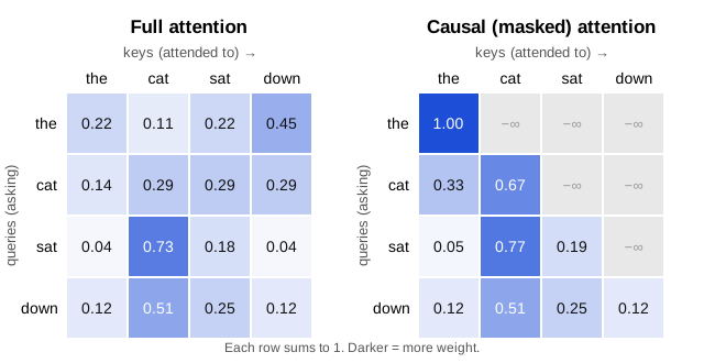
A few things jump out even in a toy. “the” spreads its attention around, with the most on “down”, because I gave “the” a query that happens to line up with the key of “down”. “cat” splits evenly between three words. Nothing forces a word to attend to itself. And nothing in the grid knows which word came first.
That last point is worth sitting on. If you shuffled the four rows of Q, K and V, you would get the same outputs, just shuffled. Attention by itself treats the sentence as a bag of words. That is why Transformers add position information to the vectors before attention ever runs. The original paper used fixed sine and cosine patterns for this.1
Why “weighted average” is the right mental model
I think the most useful way to remember attention is just: each output is a weighted average of value vectors, and the weights come from how well queries match keys.
A couple of things follow from that.
First, attention mixes. It does not compute anything fancy on its own. Since the weights are positive and sum to 1, the output for “sat” has to land somewhere between the value vectors it averaged. It cannot invent a vector outside that range. The heavy transformation happens in the feed-forward layers that sit after each attention layer, plus the learned W matrices around it.
Second, attention is about moving information between positions. Anthropic’s 2021 “mathematical framework” paper describes a Transformer as a stream of vectors that each layer reads from and adds back into, and it splits each attention head into two parts: one that decides where to look (the query-key part) and one that decides what gets copied once it looks (the value-output part).4 That split is exactly the split we saw by hand. Steps 1 to 3 were “where to look”. Step 4 was “what to copy”.
Once you see the two halves as separate, a lot of interpretability papers make more sense, because they are often asking which half is doing the interesting work.
Multi-head attention, in one paragraph
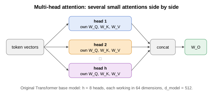
One attention operation gives each word one set of weights, which means one notion of “relevant”. But a word might need several things at once: its subject, the previous word, the matching bracket, whatever. So Transformers run several attentions side by side, each with its own W_Q, W_K, W_V, each working in a smaller space. These are heads. Their outputs are concatenated and mixed back together by one more matrix, W_O. The paper’s base model used 8 heads of 64 dimensions each, for a model width of 512, and the stated reason is that it lets the model attend to information from different representation subspaces at once.1 When people later looked at trained models, some heads really did look specialized. A 2019 study of BERT found heads that track the direct objects of verbs, determiners of nouns, and coreference, alongside many heads that mostly attend to separator tokens or the next word over.5
The causal mask
Models like GPT generate text one token at a time, left to right. When predicting the word after “sat”, the model is not allowed to peek at “down”, because at generation time “down” does not exist yet. GPT-style models are built from this kind of masked self-attention.6
The fix is simple and kind of elegant. Before the softmax, you set every score where a word would look at a later word to negative infinity. The paper describes it as masking out those illegal connections by setting them to minus infinity in the softmax input.1 Since exp(-infinity) = 0, those words get exactly zero weight, and the rest of the row renormalizes to sum to 1.
Redo “sat” with the mask. It can see “the”, “cat” and itself, but not “down”:
scaled scores: [0.00, 2.83, 1.41, -inf]
exp:           [1.00, 16.92, 4.11, 0]
total:         22.03
weights:       [0.05, 0.77, 0.19, 0.00]
“cat” gets a bit more weight than before because “down” is no longer competing. The right half of the grid figure shows the whole masked pattern. It is a triangle. The first word can only see itself, so its row is [1, 0, 0, 0] no matter what. The last word sees everything, so its row is unchanged.
The reason this matters beyond generation is training speed. With the mask in place, you can feed in a whole sentence and train the model to predict every next word at every position at the same time, in one pass, without any position cheating. That parallelism is a big part of why Transformers replaced the recurrent networks Bahdanau’s attention was originally bolted onto.
Zooming out
What attention weights are not
It is tempting to look at a grid like the one above and say “the model thinks ‘sat’ is about ‘cat’“. I did exactly that a few sections ago, and in a toy I designed, it is fair. In a real model it is a lot shakier.
Jain and Wallace showed in 2019 that attention weights often do not line up with other measures of which inputs mattered, and that quite different attention patterns can lead to the same prediction.7 Wiegreffe and Pinter pushed back the same year, arguing the answer depends on what you mean by “explanation” and how you test it.8
My read of that exchange, for what it is worth: attention weights tell you where information could have flowed, not what the model did with it. The value vectors, the output matrix, and everything downstream can make a high weight irrelevant or a low weight important. In our toy, a weight of 0.04 on a value vector that is huge could still swing the output.
So a heatmap is a good place to start asking questions. It is not an answer.
The cost
There is one more thing the hand calculation makes obvious. For four words we computed a 4 by 4 grid. For n words it is n by n. Double the length and the grid gets four times bigger.
This is not abstract for me: DebateSim had to handle long bills, which I wrote about in the paper post. Every token in a document that long has to score against every other token it can see, in every head, in every layer.
A lot of work since 2017 is about living with that grid. FlashAttention computes exactly the same result as the formula above but reorganizes the work around how GPU memory is laid out, so it never has to write the full grid out to slow memory.9 Multi-query attention shares a single set of keys and values across all the heads, which shrinks what has to be stored while generating,10 and grouped-query attention sits in between, with a few heads sharing each key-value set.11 None of these change the idea we worked out by hand. They change how cheaply you can run it.
What I’d build next
What I like about drawing attention this way is that a change in one arrow can change which words matter to another word. The arithmetic is small enough to follow, but it already gives us a way to see context changing a representation.
An interactive version could make that easier to explore. Moving a query or key would let you watch the weights shift, then see the resulting mixture move with them. I’d be curious about where that picture stops being enough: how do many heads and layers combine these simple choices into behavior that is much harder to explain?
Sources
Footnotes
-
Ashish Vaswani, Noam Shazeer, Niki Parmar, Jakob Uszkoreit, Llion Jones, Aidan N. Gomez, Łukasz Kaiser, Illia Polosukhin, “Attention Is All You Need”, NeurIPS 2017, https://arxiv.org/abs/1706.03762 ↩ ↩2 ↩3 ↩4 ↩5 ↩6
-
Dzmitry Bahdanau, Kyunghyun Cho, Yoshua Bengio, “Neural Machine Translation by Jointly Learning to Align and Translate”, arXiv 2014 (ICLR 2015), https://arxiv.org/abs/1409.0473 ↩
-
Jay Alammar, “The Illustrated Transformer”, blog post, 2018, https://jalammar.github.io/illustrated-transformer/ ↩
-
Nelson Elhage, Neel Nanda, Catherine Olsson, et al., “A Mathematical Framework for Transformer Circuits”, Transformer Circuits Thread, Anthropic, 2021, https://transformer-circuits.pub/2021/framework/index.html ↩
-
Kevin Clark, Urvashi Khandelwal, Omer Levy, Christopher D. Manning, “What Does BERT Look At? An Analysis of BERT’s Attention”, BlackboxNLP 2019, https://arxiv.org/abs/1906.04341 ↩
-
Alec Radford, Karthik Narasimhan, Tim Salimans, Ilya Sutskever, “Improving Language Understanding by Generative Pre-Training”, OpenAI, 2018, https://cdn.openai.com/research-covers/language-unsupervised/language_understanding_paper.pdf ↩
-
Sarthak Jain, Byron C. Wallace, “Attention is not Explanation”, NAACL 2019, https://arxiv.org/abs/1902.10186 ↩
-
Sarah Wiegreffe, Yuval Pinter, “Attention is not not Explanation”, EMNLP 2019, https://arxiv.org/abs/1908.04626 ↩
-
Tri Dao, Daniel Y. Fu, Stefano Ermon, Atri Rudra, Christopher Ré, “FlashAttention: Fast and Memory-Efficient Exact Attention with IO-Awareness”, NeurIPS 2022, https://arxiv.org/abs/2205.14135 ↩
-
Noam Shazeer, “Fast Transformer Decoding: One Write-Head is All You Need”, arXiv 2019, https://arxiv.org/abs/1911.02150 ↩
-
Joshua Ainslie, James Lee-Thorp, Michiel de Jong, Yury Zemlyanskiy, Federico Lebrón, Sumit Sanghai, “GQA: Training Generalized Multi-Query Transformer Models from Multi-Head Checkpoints”, EMNLP 2023, https://arxiv.org/abs/2305.13245 ↩