Why Adam won

Last week I wrote a tour of optimizers, from plain SGD to Adam to the newer stuff people are trying now. That post covered a lot of ground quickly. This one goes the other direction. I want to stay on one optimizer, Adam, and figure out why it became the thing almost everyone reaches for.

The short version is that Adam came out in 2014, and over a decade later it, or its close cousin AdamW, is still the default for training transformers. The original paper suggests lr = 0.001, beta1 = 0.9, beta2 = 0.999, eps = 1e-8 as “good default settings,”¹ and those exact numbers are still the defaults in PyTorch.² Very few things in deep learning last that long without changing.

The rest of this post is what it does differently and why that matters.

Start with the update itself

If you read my posts on what a neural network actually is and backpropagation, you saw that training is gradient descent. You compute the gradient of the loss with respect to every weight, and you nudge each weight a little bit downhill.

w = w - lr * g

Every weight gets the same lr. That is the part Adam changes.

Adam keeps two running averages for every single parameter:

m = beta1 * m + (1 - beta1) * g        # average of recent gradients
v = beta2 * v + (1 - beta2) * g * g    # average of recent squared gradients

m_hat = m / (1 - beta1 ** t)           # bias correction (more on this below)
v_hat = v / (1 - beta2 ** t)

w = w - lr * m_hat / (sqrt(v_hat) + eps)

m is momentum, the smoothed direction you have been heading. v is a running estimate of how big the gradient usually is for that parameter. Dividing by sqrt(v) means every parameter gets its own effective step size.

A parameter whose gradient is always huge gets divided by a huge number. A parameter whose gradient is always tiny gets divided by a tiny number. Both end up taking steps of roughly the same size, about lr.

That idea did not start with Adam. AdaGrad (2011) divided by the square root of the sum of all past squared gradients,³ and RMSprop, which came from a slide in Geoffrey Hinton’s 2012 Coursera course, swapped that sum for a decaying average so the step size could recover over time.⁴ Adam is basically RMSprop plus momentum plus one careful fix. The Adam paper itself says that if you remove the bias correction, what you get is RMSprop with momentum.¹

A ravine, worked out

I find the per-parameter thing hard to feel until I see it, so here is the smallest example I could think of.

Take the function f(x, y) = 0.5 * (100*x^2 + y^2). The minimum is at (0, 0). It is 100 times more curved in the x direction than in the y direction, so it looks like a long narrow ravine. Start at (1, 1).

The gradient is (100x, y). At the start that is (100, 1). Plain gradient descent has one learning rate to share between a direction where the gradient is 100 and a direction where it is 1.

If the learning rate is too large for the steep direction, x overshoots and blows up. For this function you can work out the cliff exactly: SGD on a quadratic diverges once lr passes 2 / curvature, which here is 2 / 100 = 0.02. I ran it to check. At lr = 0.019, SGD ends up at a loss of about 0.0002 after 200 steps. At lr = 0.021, the loss after 200 steps is around 10^18.

But 0.019 is a tiny learning rate for the flat y direction. Each step only shrinks y by about 2 percent. So SGD spends its time bouncing back and forth across the ravine while crawling along it.

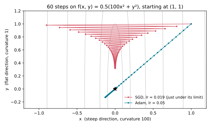
Adam’s first step is (-lr, -lr). Exactly the same size in both directions, even though the raw gradients differ by 100x, because each one got divided by its own size. It walks diagonally straight at the minimum. It does overshoot a little (it gets to about -0.13 before turning around), because momentum keeps it going. That is a real cost of Adam on a clean problem like this, and it is worth seeing.

A neural network is this ravine problem in millions of dimensions at once. Some weights sit in steep directions, some in flat ones, and you do not know in advance which is which. A single global learning rate is a compromise between all of them. Adam stops making that compromise.

Why it is robust to the learning rate

The ravine also shows the second reason people like Adam. I swept the learning rate for both optimizers on that same function, 200 steps each.

SGD   lr = 0.001  -> loss 0.34
SGD   lr = 0.01   -> loss 0.009
SGD   lr = 0.019  -> loss 0.0002
SGD   lr = 0.021  -> loss ~1.8e18   (diverged)

Adam  lr = 0.001  -> loss 33       (too slow, barely moved)
Adam  lr = 0.01   -> loss 0.012
Adam  lr = 0.1    -> loss 2.6e-9
Adam  lr = 1.0    -> loss 2.1e-8

SGD has a narrow window and then a cliff. Adam is fine across two orders of magnitude, and too small is the only way it failed here.

The Adam paper explains why. Since m_hat / sqrt(v_hat) is roughly between -1 and 1 in normal cases, the size of each step is roughly bounded by lr itself. Kingma and Ba describe this as a kind of trust region around the current weights, and they point out it means you can often guess the right scale of lr ahead of time.¹ In SGD, the step is lr * g, so the step size depends on how big your gradients happen to be, which depends on the architecture, the loss, the layer, and where you are in training.

There is a neat related fact: Adam’s update does not change if you multiply all the gradients by a constant. Scale g by c, and m scales by c while sqrt(v) also scales by c. They cancel.¹ I checked this too. Running Adam with every gradient multiplied by 1000 gave weights that matched the normal run to within about 1e-8, which is just the eps term leaking through.

A quick caveat so I do not oversell this. My sweep is one toy quadratic. In real training the learning rate is still the hyperparameter you tune first, Adam included. “Robust” here just means the good range is wide and the failure is gentler. You still tune it.

Bias correction, the step people skip

This is the one line in Adam that I did not understand the first time I saw it.

m and v both start at zero. Look at what happens in the first few steps if the gradient is exactly 1.0 every time. With beta1 = 0.9, after step one m = 0.1. After step two, m = 0.19. The true average gradient is 1, but the running average is stuck way below it because it is still partly made of the zeros it started from.

v is even worse, because beta2 = 0.999 decays so slowly. After step one, v = 0.001.

Now here is the trap. If you skip correction and compute m / sqrt(v), you get 0.1 / sqrt(0.001), which is about 3.16. Your first step is more than three times lr. It peaks at about 6.5 times lr around step 12, and it is still about 4.5 times lr at step 50. Both averages are biased low, but v is biased much lower, and it sits under a square root in the denominator, so the whole thing blows up.

The fix is the division by 1 - beta ** t. At step one, 1 - 0.9 = 0.1, so m_hat = 0.1 / 0.1 = 1.0. Same for v. Both corrected averages land on the true value from the very first step.

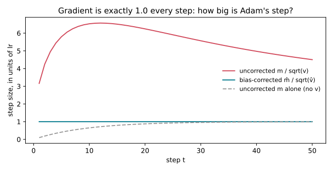
The Adam paper says this matters most when beta2 is close to 1, which is exactly the setting you want for sparse gradients, and in their experiments leaving it out caused instability early in training.¹ The first steps are when the weights are random and the gradients are wild, so it is the worst possible time to accidentally take a 6x step.

Adam in about 15 lines of NumPy

Here is the whole thing. This is what I used for the plots and the numbers above.

import numpy as np

def adam(grad, x, lr=1e-3, b1=0.9, b2=0.999, eps=1e-8, steps=1000):
    m = np.zeros_like(x)          # running average of gradients
    v = np.zeros_like(x)          # running average of squared gradients
    path = [x.copy()]
    for t in range(1, steps + 1):
        g = grad(x)
        m = b1 * m + (1 - b1) * g
        v = b2 * v + (1 - b2) * g * g
        m_hat = m / (1 - b1 ** t)  # bias correction
        v_hat = v / (1 - b2 ** t)
        x = x - lr * m_hat / (np.sqrt(v_hat) + eps)
        path.append(x.copy())
    return np.array(path)

H = np.array([100.0, 1.0])                  # the ravine
path = adam(lambda p: H * p, np.array([1.0, 1.0]), lr=0.1, steps=200)
print(path[-1])                             # very close to [0, 0]

Notice the memory cost while you are here. For every parameter, Adam stores two extra numbers, m and v. A model with a billion weights carries two billion extra numbers of optimizer state. That is one of the reasons people keep trying to build something cheaper, which I got into in the survey post.

The sign-descent view

This is the part that changed how I picture Adam.

Set beta1 = 0 and make beta2 tiny, so m is just the current gradient and v is just the current squared gradient. Then the update is g / sqrt(g^2) = g / |g|, which is +1 or -1. That is sign descent: ignore how big the gradient is, only look at which way it points, and step by lr in that direction. There is a whole line of work on it, including signSGD.⁵

Real Adam is not that extreme, but Balles and Hennig showed that it is close in a precise way. They split Adam’s update into two pieces: the sign of the gradient, which picks the direction, and a magnitude that depends on how noisy the gradient is relative to its size.⁶

You can see it with a little algebra. If the average gradient for a weight is mu and its noise has variance sigma^2, then m is roughly mu and v is roughly mu^2 + sigma^2. So:

m / sqrt(v)  ≈  mu / sqrt(mu^2 + sigma^2)
             =  sign(mu) * 1 / sqrt(1 + sigma^2 / mu^2)

When the gradient is consistent (low noise), the second factor is close to 1 and Adam takes a full sign step. When the gradient is mostly noise, the factor shrinks and Adam steps carefully. Kingma and Ba actually say the same thing in their own paper: they call m_hat / sqrt(v_hat) a signal-to-noise ratio and note that it naturally shrinks near an optimum, a kind of automatic annealing.¹

So my mental picture of Adam now is: sign descent, with a built-in brake for noisy directions. Balles and Hennig went further and argued that the sign part is what hurts Adam’s generalization on some tasks, not the variance part.⁶ That lines up with an older finding by Wilson and others that adaptive methods could generalize worse than well-tuned SGD on several image benchmarks.⁷ That’s part of why SGD with momentum hung on so long in computer vision.

Why it wins on language specifically

So if sign descent sometimes generalizes worse, why does Adam beat SGD so clearly on transformers and language models?

The first guess people had was noise. Zhang and others argued in 2020 that gradient noise in attention models is heavy-tailed, with occasional huge gradients, and that adaptive methods handle that better than SGD.⁸ That sounds right. But in 2023, Kunstner, Chen, Lavington and Schmidt tested it directly by growing the batch size all the way to the full dataset, which removes the noise. The gap did not close. Adam actually got better as noise went down, while SGD gained less. And full-batch Adam behaved a lot like sign descent with momentum.⁹ So noise was not the main story.

Their follow-up in 2024 is the explanation I find most convincing.¹⁰ Language has heavy-tailed class imbalance. When a model predicts the next token, each token in the vocabulary is a class, and a handful of tokens (“the”, ”,”, ”.”) show up constantly while tens of thousands of others are rare. The rare ones are each uncommon, but together they make up a big chunk of the data.

With plain gradient descent, the gradient for a rare token’s weights is small, because that token rarely appears. So those weights barely move, and the loss on rare tokens drops very slowly. Slow learning on the long tail can then hold back the average loss too. Adam divides each parameter’s gradient by its own typical size, so a rare token’s small gradient gets scaled up to a normal-sized step. The authors show the same effect in vision models and even linear models once they make the classes heavy-tailed, and they prove that in a simplified continuous-time setting, gradient descent is slow on rare classes while sign descent is not.¹⁰

This connects straight back to the ravine. Rare tokens are the flat direction. Common tokens are the steep one. SGD’s one learning rate has to be small enough for the steep part, and the flat part pays for it.

I do not think this is the whole story. It is one convincing piece of it, and it is the piece that explains why the Adam advantage is so specific to language.

Weight decay, done right: AdamW

The last piece is the one that turned Adam into AdamW, which is what most people actually use now. I covered decoupled weight decay in the survey post; the short version is that putting an L2 penalty into Adam’s gradient lets sqrt(v) rescale the decay, so AdamW applies it to the weights directly.¹¹

You can see the distinction in PyTorch. With Adam’s default decoupled_weight_decay=False, a nonzero decay is added to the gradient (g = g + lambda * theta). Setting it to True gives AdamW behavior. The separate torch.optim.AdamW class uses decoupled decay and defaults to weight_decay=0.01, while Adam defaults to zero.²¹² The class and configuration both matter.

So why did it win

Adam makes sense to me as a practical choice because it adjusts updates using the history of each parameter’s gradients. The original transformer used it too.¹³ That doesn’t make it the best choice for every model, but it helps explain why it became such a familiar starting point.

What interests me now is how much of an optimizer’s apparent advantage comes from the method and how much comes from knowing how to tune it. I’d like to compare methods with the same budget and look at where their behavior differs, especially on parameters that get useful signals less often. A better default could make training easier, but understanding when to leave that default behind seems just as useful.

Sources