A common pattern in transformers is a line of code repeated dozens of times: x = x + layer(x). Take the running vector, compute something, add it back. That plus sign is the residual connection, and ResNet helped make it a standard ingredient of deep networks in 2015.1
In March 2026 the Kimi team at Moonshot AI put out a paper called “Attention Residuals” that asks a simple question about that plus sign: why is every weight in it equal to 1?2 Their answer is to replace the fixed sum with attention over depth, so each layer gets to choose which earlier layers it reads from. They trained it into a 48B-parameter model and it matched or beat the baseline on every benchmark they reported.
I want to go through the paper carefully, because I think the interesting part is not only the benchmark gains. It is that the change gives you a small, explicit, readable record of how information moves through depth. That seems worth exploring for interpretability.
A note on attribution, since I am calling it “the Moonshot AI paper” in the title. The arXiv listing names the authors as the Kimi Team plus 36 individual researchers, and the official code lives under the MoonshotAI organization on GitHub.23 Kimi is Moonshot AI’s model family, and alphaXiv lists the authors with Moonshot AI as their affiliation.4
The plus sign, unrolled
Start with what a normal residual stream actually computes. Write h_l for the vector entering layer l, and f_l for what layer l does (an attention block or an MLP; the paper counts each as its own “layer”).
h_l = h_{l-1} + f_{l-1}(h_{l-1})If you unroll that recurrence, you get this:
h_l = h_1 + f_1(h_1) + f_2(h_2) + ... + f_{l-1}(h_{l-1})The input to any layer is the embedding plus every earlier layer’s output, all added with weight exactly 1. Layer 40 cannot say “I mostly care about what layer 3 found.” It gets one blended vector, and whatever layer 3 wrote is in there somewhere, mixed with 39 other contributions.
I wrote about this view of the residual stream in How a word gets meaning inside a model, where the stream is a shared channel that every layer reads from and writes to. In my read of Attention Is All You Need I also called residuals the part of the architecture I think about most. So this paper hit a nerve.
The paper names three problems with the fixed sum.2 First, every layer gets the same blended state, with no way to weight its sources differently. Second, once information is blended in, a later layer cannot pull it back out cleanly. Third, and this is the measurable one, the stream keeps growing.
Why the stream keeps growing
Most modern models use pre-norm: normalize the input to each layer, but leave the residual path itself untouched.5 That is good for training stability, because the identity path carries gradients straight through. The cost is that nothing ever shrinks the stream. Each layer adds to it, so its magnitude grows roughly linearly with depth.26
Now think about layer 50. Its input gets normalized, so it sees a fixed-scale vector. Its output gets added to a stream that is already huge. To change the stream noticeably, layer 50 has to produce a large output. The paper calls this PreNorm dilution: each layer’s relative contribution shrinks as you go deeper, and later layers compensate by learning bigger and bigger outputs.2
There is outside evidence that deep layers are underused. Gromov and colleagues found that you can prune a large fraction of the deeper layers of open models with surprisingly little loss on question-answering benchmarks.7 The AttnRes paper cites that result as a symptom of the same problem.2
The fix: attention, but over layers
The paper’s framing is the part I liked most. An RNN squeezes the whole past sequence into one hidden state, one step at a time. A residual stream squeezes the whole past depth into one hidden state, one layer at a time. Transformers fixed the RNN problem by letting each position attend over all previous positions directly. So: let each layer attend over all previous layers directly.2
Here is the AttnRes update:
h_l = sum over i from 0 to l-1 of  alpha_{i->l} * v_i

v_0 = h_1             (the token embedding)
v_i = f_i(h_i)        (layer i's output), for i >= 1
The weights alpha_{i->l} come from a softmax, so they are positive and sum to 1. If you already know how normal attention works (I drew it out step by step in Attention, drawn by hand), the pieces map over like this:
- Query: a single learned vector
w_lper layer. The paper calls it a pseudo-query, because it does not depend on the input. It is just a parameter. - Keys: the earlier outputs themselves, passed through RMSNorm. So
k_i = RMSNorm(v_i). - Values: the earlier outputs, unnormalized.
score_i  = w_l · RMSNorm(v_i)
alpha_i  = exp(score_i) / sum_j exp(score_j)
The query is fixed, but the keys depend on the actual content of each earlier output for this token. So the weights still change from token to token. That is the “input-dependent” part.
The RMSNorm on keys matters. Without it, a layer that happens to produce large outputs would win the softmax just by being loud. The ablations show that removing it hurts.2
A tiny worked example
Say layer 4 is choosing among four sources: the embedding and layers 1, 2 and 3. Suppose its pseudo-query produces scores [1.0, -0.5, 0.2, 2.0]. The softmax turns those into roughly:
embedding  0.228
layer 1    0.051
layer 2    0.102
layer 3    0.619
Layer 4 now reads mostly from layer 3, takes a real chunk of the raw embedding, and nearly ignores layer 1. A standard residual would have given all four a weight of 1.
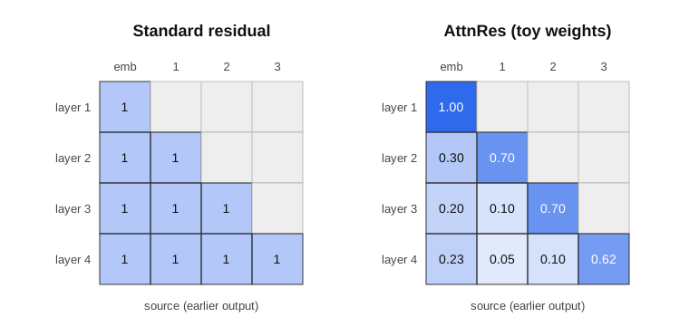
One detail I would have missed on a skim: all pseudo-queries are initialized to zero. With a zero query, every score is 0, so the softmax is uniform and AttnRes starts out as a plain average of earlier outputs. The authors say this initialization is required and that it prevents training instability.2 Notice it is an average, not a sum. That alone keeps the input bounded, which is part of how it fights dilution.
The extra parameters are tiny: one d-dimensional query and one RMSNorm per layer.2
Full vs. Block AttnRes
The version above, where every layer can attend to every earlier output, is Full AttnRes. The arithmetic is cheap, since depth is in the tens or hundreds and attention over that is nothing compared to attention over a long context. The problem is systems. In ordinary training you keep layer outputs around for backprop anyway, so there is no extra memory.2 At scale, people recompute activations instead of storing them and split layers across machines with pipeline parallelism. Full AttnRes forces every layer output to stay alive and get shipped across machine boundaries. That is O(L·d) memory and communication per token.
Block AttnRes is the practical version. Split the L layers into N blocks. Inside a block, outputs are summed the normal way. Across blocks, each layer attends over the N block summaries plus the embedding, plus the running partial sum of the current block.2 Set N = L and you get Full AttnRes back. Set N = 1 and you get roughly a standard residual. They found N around 8 recovers most of the benefit.
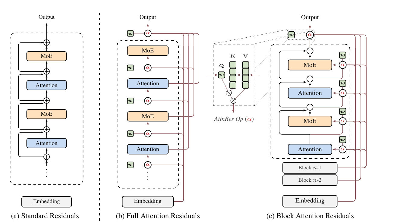
There is a whole section on infrastructure: caching block summaries across pipeline stages so they are not resent, and a two-phase inference trick where all the layers in a block batch their cross-block attention into one pass and then merge it with the in-block part using online softmax.2 The reported cost is under 4% end-to-end training overhead with pipeline parallelism, and under 2% inference latency on typical workloads.2 I can’t check those numbers myself, but the design reasons for them hold together.
What the experiments show
Scaling
They trained five model sizes, from 194M to 528M activated parameters, each as a baseline, Full AttnRes and Block AttnRes, using hyperparameters tuned for the baseline.2 That choice favors the baseline, which makes the comparison more convincing. AttnRes had lower loss at every size. On the fitted curves, Block AttnRes matches a baseline trained with 1.25 times more compute. At the largest size, Full and Block differ by just 0.001 in validation loss (1.692 vs. 1.693).2
The big model
The main run uses the Kimi Linear architecture, a mixture-of-experts model with 48B total and 3B active parameters, 54 layers, and a mix of linear-attention and full-attention blocks.82 They used Block AttnRes with 6 layers per block, which gives 9 blocks plus the embedding, so 10 sources to attend over. Pre-training was 1T tokens followed by about 400B tokens of mid-training.2
Against the same recipe without AttnRes, it matched or beat the baseline on all 15 benchmarks in their table. MMLU-Pro was a tie at 52.2. Some of the bigger gaps:2
| Benchmark | Baseline | AttnRes |
|---|---|---|
| GPQA-Diamond | 36.9 | 44.4 |
| Math | 53.5 | 57.1 |
| HumanEval | 59.1 | 62.2 |
| C-Eval | 79.6 | 82.5 |
| MMLU | 73.5 | 74.6 |
The authors read the bigger gains on multi-step reasoning and code as support for the idea that later layers benefit from pulling specific earlier results back up.2 That is plausible, but it is a hypothesis. It is one training run per arm, and a 7.5-point jump on GPQA-Diamond, a small benchmark, is the kind of number I would want to see replicated before leaning on it.
The training dynamics plots show what you would hope. In the baseline, output magnitude climbs with depth and gradients pile up in the earliest layers. With Block AttnRes, magnitudes stay bounded in a repeating pattern that resets at each block boundary, and gradients spread out more evenly.2
The ablations
This is where the paper earns trust, I think. On the 16-block model (16 attention plus 16 MLP layers, baseline loss 1.766), with everything else held fixed:2
- DenseFormer, which also lets each layer see all earlier outputs but with fixed learned scalar weights, gets 1.767. No gain.9 In this comparison, access to earlier layers alone did not improve loss. The input-dependent weights seem important.
- mHC, a recent method from DeepSeek that keeps several parallel residual streams with learned mixing, gets 1.747.10
- Full AttnRes: 1.737. Block AttnRes (block size 4): 1.746.
- Replacing the query and keys with input-independent scalar weights: 1.749.
- Sigmoid instead of softmax: 1.741. They credit softmax’s competition between sources for sharper selection.
- Removing RMSNorm on keys: 1.743 (Full), 1.750 (Block).
- A sliding window over only the 8 most recent layers plus the embedding: 1.764, barely better than baseline. Reaching far back matters more than seeing many nearby layers.
- Making the query depend on the current hidden state: 1.731, the best number in the table. They skip it anyway, because it adds a
d × dprojection per layer and breaks the batching trick at inference. - Per-head depth weights (16 heads): worse, 1.752 vs. 1.746. Splitting the routing by head did not help in this setup.
The input-dependent query result is the one I find most interesting. The best version was set aside for systems reasons, which means the gains in the paper are probably not the ceiling.
There is also an architecture sweep at fixed compute. AttnRes won in all 25 width and depth settings they tried, and its best setting was deeper and narrower than the baseline’s.2 The authors are careful to say this is a diagnostic, not a recommendation, since deeper models are slower at inference.
What the routing looks like
This is the figure I spent the most time on.
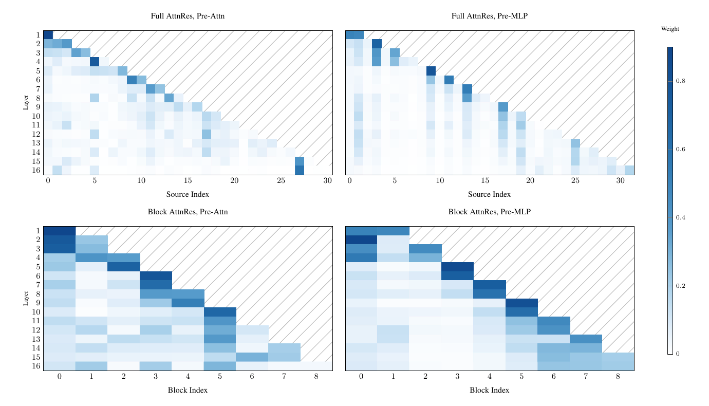
Three patterns, as the paper describes them:2
- Mostly local. The darkest cells sit right next to the diagonal. Each layer leans hardest on the one just before it, so the ordinary residual path is still doing most of the work.
- The embedding never goes away. Column 0, the raw token embedding, keeps getting real weight all the way up, especially in the inputs to attention layers.
- Occasional long jumps. A few bright cells far from the diagonal: layer 4 reaching back to early sources, and in the Block version layers 15 and 16 reaching back several blocks. Those are learned skip connections the model built for itself.
They also note a split: inputs to MLPs stick closer to the diagonal, while inputs to attention layers spread their weight more widely. That fits a picture where attention moves information around and MLPs work locally. In the discussion section they mention depth-wise attention sinks, layers that soak up weight no matter the input, which mirrors the attention sinks people found over sequences.211
One caveat that matters for what comes next: these heatmaps are averages over tokens. The paper does not show per-token routing.
My take: a depth channel you can actually read
What interests me beyond the benchmark table is what this might let us inspect.
A lot of interpretability work starts from the residual stream being a shared channel that every layer reads and writes.12 The trouble is that in a normal model, the channel is a sum. If you want to know whether layer 30 used something layer 5 wrote, you have to infer it: project the stream through the unembedding to see what it predicts at each depth (the logit lens and its trained successor, the tuned lens), or trace circuits by hand.1314 The reading-from-earlier-layers step is implicit.
In AttnRes, that step is a number. For every token, every layer emits a probability distribution over its sources, and the model has to compute it anyway. You get a per-token map of which earlier states each layer chose to read, for free. That is a depth-wise routing signal sitting in plain sight, the same way attention patterns over tokens became a first stop for interpretability research.
I don’t want to oversell it. Attention weights are not explanations by default. Jain and Wallace showed years ago that token-level attention weights can be shuffled or swapped without changing a model’s output much, so a high weight does not prove that source caused the result.15 The same worry applies here, with a twist: keys are normalized but values are not, so a source with weight 0.1 and a huge norm could still contribute more than a source with weight 0.4. Any real analysis should look at alpha × ||v||, not alpha alone. And in Block AttnRes, everything inside a block is summed, so you can see which block a layer reached back to, but not which layer inside it.
Still, it changes what experiments are cheap. The one I would want to run is about revisiting. When a model hits something inconsistent partway through a problem, like a step in a math solution that contradicts an earlier one, does it reach back to earlier states? You could take a small AttnRes model, along the lines of the paper’s 16-layer setup, and build pairs of inputs that are identical except that one has a planted contradiction. Then compare the routing at the positions after the contradiction. If later layers shift weight toward the embedding or toward early blocks on the inconsistent inputs, that is a measurable signature of a model “rechecking” its earlier representation of the problem. If nothing moves, that is informative too.
I don’t fully know yet whether that signal would be there. The averaged heatmaps say the model mostly reads locally, and averages can hide exactly the rare, input-specific jumps I would be looking for. But I like that the question is now a matter of logging a tensor the forward pass already computes. Before this, it was a research project in itself.
What I’m taking from it
What excites me about this paper is that it gives the model a different way to use earlier layers, and gives us another set of choices to inspect.2 I’d like to know whether those choices help explain what happens when the model changes its answer or gets stuck.
The weights alone won’t answer that. But we could change which earlier states are available and watch whether the output changes in a way we can explain. If that works, depth routing could become useful for understanding a model as well as improving it. That’s the possibility I want to follow beyond the benchmark table.
Sources
Footnotes
-
Kaiming He, Xiangyu Zhang, Shaoqing Ren, Jian Sun, “Deep Residual Learning for Image Recognition”, CVPR 2016 (arXiv 2015), https://arxiv.org/abs/1512.03385 ↩
-
Kimi Team (Guangyu Chen, Yu Zhang, Jianlin Su, et al.), “Attention Residuals”, arXiv 2603.15031, March 2026, https://arxiv.org/abs/2603.15031 ↩ ↩2 ↩3 ↩4 ↩5 ↩6 ↩7 ↩8 ↩9 ↩10 ↩11 ↩12 ↩13 ↩14 ↩15 ↩16 ↩17 ↩18 ↩19 ↩20 ↩21 ↩22 ↩23 ↩24 ↩25 ↩26
-
MoonshotAI, “Attention-Residuals” official repository, GitHub, 2026, https://github.com/MoonshotAI/Attention-Residuals ↩
-
alphaXiv listing for “Attention Residuals” (author affiliations), https://www.alphaxiv.org/abs/2603.15031 ↩
-
Ruibin Xiong et al., “On Layer Normalization in the Transformer Architecture”, ICML 2020, https://arxiv.org/abs/2002.04745 ↩
-
Tianyu Li et al., “SiameseNorm: Breaking the Barrier to Reconciling Pre/Post-Norm”, arXiv 2602.08064, 2026, https://arxiv.org/abs/2602.08064 ↩
-
Andrey Gromov et al., “The Unreasonable Ineffectiveness of the Deeper Layers”, arXiv 2403.17887, 2024, https://arxiv.org/abs/2403.17887 ↩
-
Yu Zhang et al., “Kimi Linear: An Expressive, Efficient Attention Architecture”, arXiv 2510.26692, 2025, https://arxiv.org/abs/2510.26692 ↩
-
Matteo Pagliardini et al., “DenseFormer: Enhancing Information Flow in Transformers via Depth Weighted Averaging”, arXiv 2402.02622, 2024, https://arxiv.org/abs/2402.02622 ↩
-
Zhenda Xie et al., “mHC: Manifold-Constrained Hyper-Connections”, arXiv 2512.24880, 2025, https://arxiv.org/abs/2512.24880 ↩
-
Guangxuan Xiao et al., “Efficient Streaming Language Models with Attention Sinks”, arXiv 2309.17453, 2023, https://arxiv.org/abs/2309.17453 ↩
-
Nelson Elhage et al., “A Mathematical Framework for Transformer Circuits”, Transformer Circuits Thread (Anthropic), December 2021, https://transformer-circuits.pub/2021/framework/index.html ↩
-
nostalgebraist, “interpreting GPT: the logit lens”, LessWrong, 2020, https://www.lesswrong.com/posts/AcKRB8wDpdaN6v6ru/interpreting-gpt-the-logit-lens ↩
-
Nora Belrose et al., “Eliciting Latent Predictions from Transformers with the Tuned Lens”, arXiv 2303.08112, 2023, https://arxiv.org/abs/2303.08112 ↩
-
Sarthak Jain and Byron C. Wallace, “Attention is not Explanation”, NAACL 2019, https://arxiv.org/abs/1902.10186 ↩